The Exchange Economy
In a lecture on microeconomics, the analysis of an exchange economy consisting of two consumers is usually the first step towards general equilibrium theory. This step from partial to general equilibrium analysis is larger than it appears at first glance, because prices and income are no longer exogenously given, but result from market events. The decision of the one depends on the decision of the other. Thus, the mathematics of equilibrium is of a different kind than what one is used to from partial analysis, and it is important to understand the basic principles of the exchange economy of two consumers mathematically and economically from the outset.
When I wanted to mathematically thoroughly understand an Edgeworth box in I. M. D. Little's great dissertation A Critique of Welfare Economics
, I had to concede deficits in mathematical and economic understanding and not only refresh my knowledge of the concept of an exchange economy, but deepen and complement it. This is the cause for this article. Its aim is to present the theory of general equilibrium, which is central to microeconomics, up to the First Theorem of Welfare Economics, using the simple case of an exchange economy with two persons and two goods, in such a way that an understanding of the core of the theory can be achieved, making it easier to grasp all the contents beyond it. I hope this presentation will be enlightening for some students of economics. For the economically interested layman the article Basic Terms of Microeconomics
offers a propaedeutic introduction to the prerequisite terms and concepts.
Contents
1. The Mathematical Model
2. Market Equilibrium and Pareto Efficiency
3. The Marginal Rate of Substitution and Pareto Efficiency
4. The Derivation of the Contract Curve
5. Individual Utility Maximization and Demand Functions
6. Walras' Law, Excess Demand and the Relativity of Prices
7. The General Equilibrium
8. The Justification of Market Equilibrium
9. The First Theorem of Welfare Economics
10. Digression: Edgeworth and the Perfection of the Markets
11. Final Remarks
References
1. The Mathematical Model
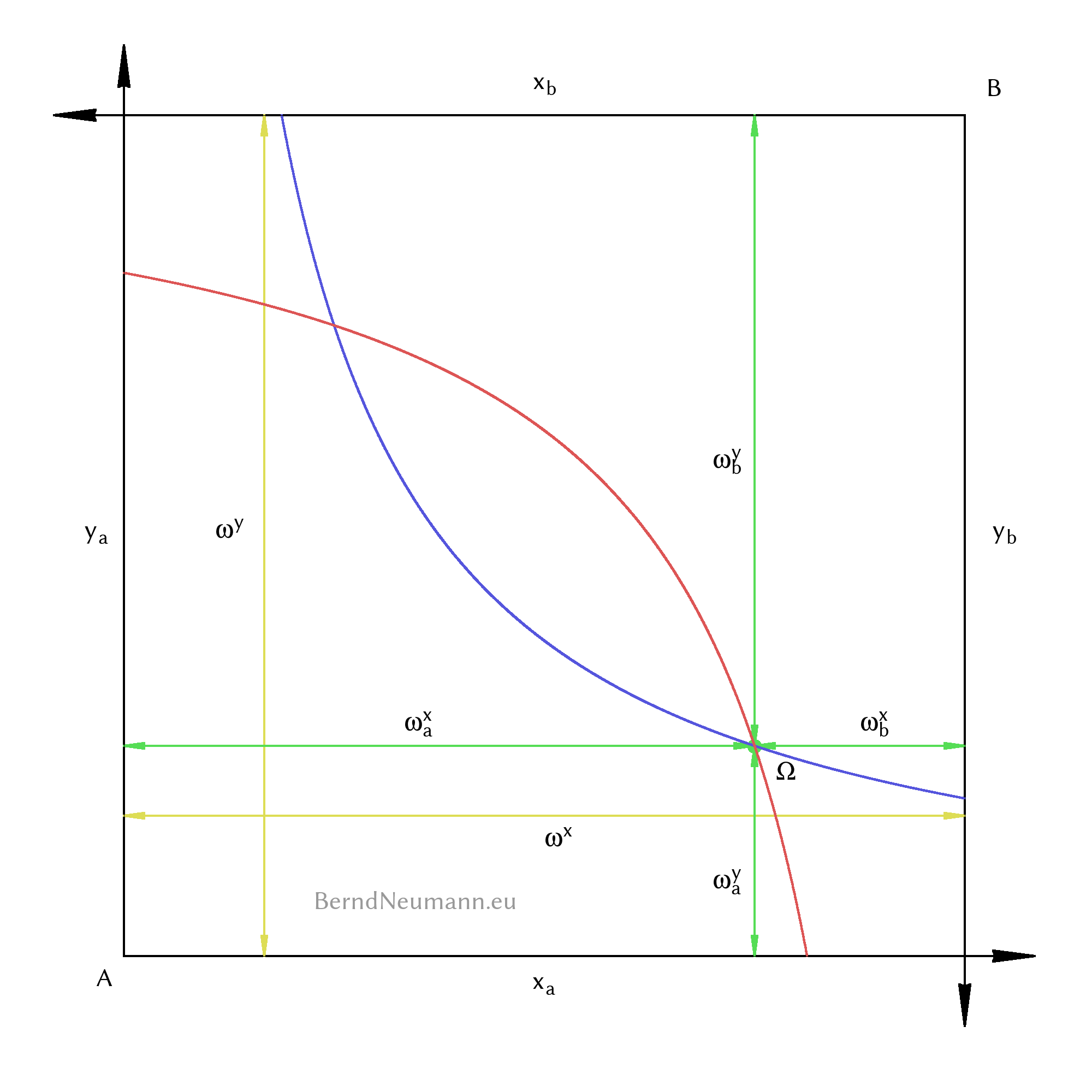
We define the functions and variables of the exchange economy at the beginning: There are two individuals \(A\) and \(B\) who exchange two goods \(X\) and \(Y\). The amount that individual \(A\) consumes of good \(X\) is called \(x_a\); the amount that \(A\) consumes of good \(Y\) is called \(y_a\). For individual \(B\) we name these quantities of goods accordingly \(x_b\) and \(y_b\). The individuals have the Cobb-Douglas utility functions $$\begin{aligned} U_a(x_a, y_a) \; &= \; x_a^\alpha \; y_a^{(1-\alpha)} \qquad \text{with } \alpha \in [0;1]\\[0.5em] U_b(x_b, y_b) \; &= \; x_b^\beta \; y_b^{(1-\beta)} \qquad \text{with } \beta \in [0;1] \end{aligned}$$
In the economy there is a total endowment \(\omega^x\) of good \(X\) and \(\omega^y\) of good \(Y\). Individual \(A\) initially has \(\omega^x_a\) units of good \(X\) and \(\omega^y_a\) units of good \(Y\). We call the initial endowment of individual \(B\) accordingly \(\omega^x_b\) and \(\omega^y_b\). The point of the initial endowment in the edgeworth box we call \(\Omega\). Note that the initial endowment is exogenous, while the quantities consumed \(x_a \), \(x_b \), \(y_a\) and \(y_b\) are endogenous variables.
There is no production and no goods are thrown away in the exchange economy. We therefore have the feasibility condition:$$\begin{aligned} \omega^x \; &= \; \omega^x_a \,+\, \omega^x_b \; = \; x_a \,+\, x_b\\[0.5em] \omega^y \; &= \; \omega^y_a \,+\, \omega^y_b \; = \; y_a \,+\, y_b \end{aligned}$$
The following Edgeworth box illustrates these definitions:
2. Market Equilibrium and Pareto Efficiency
In the Edgeworth box of an exchange economy two concepts are presented. On the one hand, there are markets on which goods are offered and demanded at certain prices. If supply equals demand on all markets, we speak of a general equilibrium. This part of the theory describes the result of individual actions on the markets. On the other side is Pareto efficiency. An allocation is Pareto efficient if you cannot make someone better off without making someone else worse off. In other words, a Pareto efficient allocation does not waste the opportunity to improve people's welfare through exchange. This part of the theory explains which allocations are desirable.
It is important to distinguish clearly between these two parts. This may seem trivial or even unrealistic in an exchange economy with only two people and two goods, but the point is not to explain the actions of two people on a desert island with two goods, but the simple two-person case stands for markets with many participants operating under perfect competition. How both parts are related is the punch line at the end in the form of the First Theorem of Welfare Economics. It becomes meaningless if the parts are carelessly mixed up beforehand.
In the following sections I will explain both concepts one after the other. The aim is not to arrive at the First Theorem of Welfare Economics in the shortest and most direct way possible, but to explain the mathematics and its economic meaning in detail and to illustrate it with appropriate graphics. We start with Pareto efficient allocations by using the Edgeworth box to examine the meaning of the marginal rate of substitution.
3. The Marginal Rate of Substitution and Pareto Efficiency
In partial equilibrium analysis, it is as illustrative as it is sufficient to understand the marginal rate of substitution as the slope of the indifference curves. For the general equilibrium analysis it is more descriptive to think of it as a scalar field like the utility functions. Instead of the utility value, the function of the marginal rate of substitution provides a scalar for each allocation, which expresses the willingness to exchange. Willingness to exchange means, that for a marginal unit of one good, one is willing to give away at most a certain amount of the other good. Let us take this view from the beginning: We have the utility functions, which we draw as indifference curves in the Edgeworth box. In reality, the utility function is three-dimensional, and the indifference curves are their contour lines in the two-dimensional Edgeworth box. If an exchange lies on a contour line and thus corresponds exactly to the willingness to exchange, the utility level remains constant. The difference of utility before and after the exchange is zero: $$\begin{aligned} \Delta U(x, y) \; &= \; 0 \end{aligned}$$
In order for this to be fulfilled, the following must happen during an exchange: One gets from a good, let us say it is good \(X\), a marginal unit \({\text d}x\) in addition. By this movement in \(x\)-direction the utility changes according to the slope in this direction. This slope of the utility function is its partial derivative of \(x\). In order for \(\Delta U\) to remain zero, we must compensate this utility gain by a corresponding movement \({\text d}y\). This movement in \(y\)-direction must be weighted with the slope of the utility function in \(y\)-direction. The sum of these two movements, which we have considered in simple plus-minus arithmetic, is the total differential of the utility function \(\Delta U(x, y)\): $$\begin{aligned} \Delta U(x, y) \; = \; \frac{\partial U(x, y)}{\partial x}{\text d}x \; + \; \frac{\partial U(x, y)}{\partial y}{\text d}y \; &= \; 0 \end{aligned}$$
By rearranging one obtains: $$\begin{aligned} \frac{{\text d}y}{{\text d}x} \; &= \; -\frac{\frac{\partial U(x, y)}{\partial x}}{\frac{\partial U(x, y)}{\partial y}} \end{aligned}$$
The left part of this equation reads as follows: For the utility to remain constant, \(\Delta U = 0\), \(y\) must change by \({\text d}y\) when \(x\) changes by \({\text d}x\). On the right side of the equation are the partial derivatives, which are always positive because of the monotony. Because of the minus sign, the right part is always negative. This means that on the left side \({\text d}x\) and \({\text d}y\) must have different signs. This means economically, that you would give something of good \(Y\), if you gain a marginal unit of good \(X\) and the utility shall remain constant. This quantity, which one would give away of good \(Y\), is the (negative) slope of the indifference curve and nothing else as the marginal rate of the substitution.
We call the marginal rate of substitution \(\text{MRS}^x\) and write it as a function \(\text{MRS}^x(x, y)\). The superscript \(x\) reminds us that we transformed the total differential to \(\frac{{\text d}y}{{\text d}x}\). To express the willingness to exchange as units of good \(Y\) per unit of good \(X\) is arbitrary, because we could have also converted to \(\frac{{\text d}x}{{\text d}y}\). It is important to choose a reference good and to keep it for all individuals. With the equation from the total differential we can calculate the function of the marginal rate of substitution for both individuals by forming and using the partial derivatives: $$\begin{aligned} \text{MRS}_a^x(x_a, y_a) \; &= \; -\;\frac{\alpha x_a^{(\alpha-1)}y_a^{(1-\alpha)}}{x_a^\alpha (1-\alpha)y_a^{(1-\alpha-1)}}\\[1em] \text{MRS}_a^x(x_a, y_a) \; &= \; -\; \frac{\alpha}{1-\alpha} \frac{y_a}{x_a}\\[1em] \text{MRS}_b^x(x_b, y_b) \; &= \; -\; \frac{\beta}{1-\beta} \frac{y_b}{x_b} \end{aligned}$$
With the equations for the marginal rate of substitution we can formulate the optimality condition for the Pareto efficient allocations. An allocation is Pareto efficient if nobody can be made better off without making someone else worse off. This is the case if the marginal rate of substitution is equal for both individuals. Assuming it is not equal, one of them would be willing to pay more good \(Y\) for a marginal unit of good \(X\) than the other one needs to give a marginal unit of good \(X\) at constant level of utility. This difference could be used to make one or both better off, so that the initial allocation cannot have been Pareto efficient.
The following two figures illustrate this relationship with \(\alpha = \frac{2}{5}\) and \(\beta = \frac{3}{5}\). Here, Figure 3a provides the mathematically intuitive view by representing the \(\text{MRS}^x\) as a scalar field that expresses the willingness to exchange. Figure 3b corresponds to the usual economic view. In it the lenticular common better set shows the possibility to make at least one better off without having to make the other worse off. A Pareto efficient allocation is only achieved if the indifference curves are just touching each other, i.e. if their slopes, i.e. the marginal rate of substitution of both individuals, are equal for an allocation.
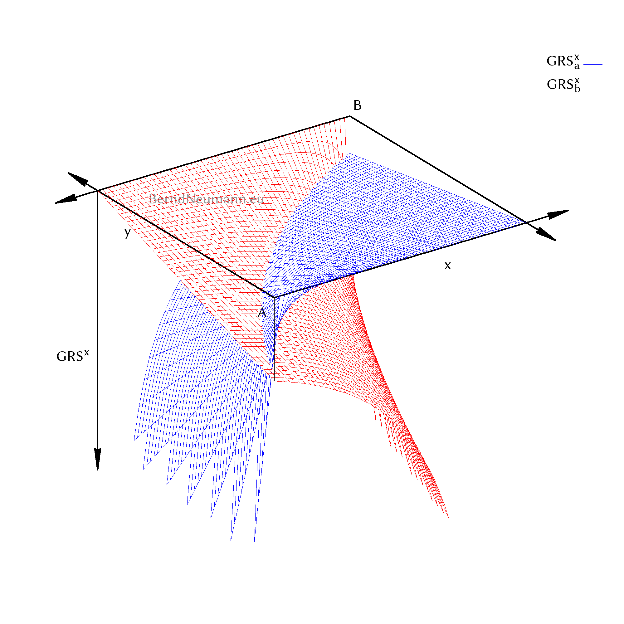
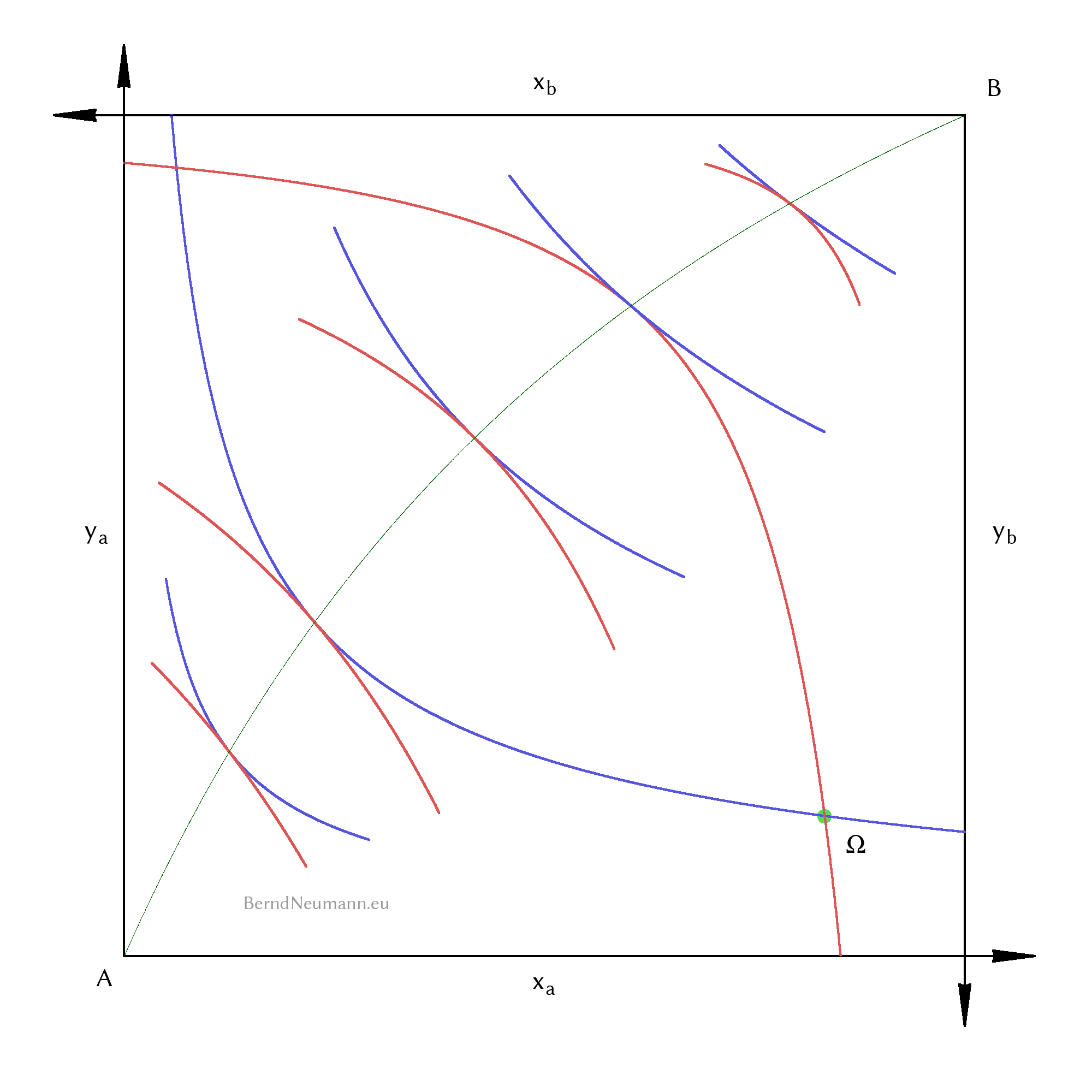
Point on the Contract Curve.
Both illustrations show the obvious: In Pareto efficient allocations, the marginal rate of substitution of the individuals is the same. Both illustrations have advantages and disadvantages. The usual representation with the indifference curves makes it clear whether or not someone can be made better off. This illustrates the economic significance of Pareto efficiency, which we want to get to with the marginal rate of substitution. However, the mathematical point of view takes a back seat. A look at the indifference curves and their slopes obscures the fact that the marginal rate of substitution is a function that expresses the individual's willingness to exchange for a certain allocation. This mathematical view is clearer if the marginal rate of substitution is written as a function and represented three-dimensionally as a scalar field.
4. The Derivation of the Contract Curve
We are looking for the set of Pareto efficient allocations and want to derive the equation of the contract curve. In the previous section, we calculated the \(\text{MRS}^x\) for both individuals and showed that in Pareto efficient allocations, the marginal rates of substitution must be equal. Equating and substituting gives: $$\begin{aligned} \text{MRS}_a^x(x_a, y_a) \; &= \; \text{MRS}_b^x(x_b, y_b)\\[1em] \frac{\alpha}{1-\alpha} \frac{y_a}{x_a} \; &= \; \frac{\beta}{1-\beta} \frac{y_b}{x_b} \end{aligned}$$
We now have an equation with four variable quantities of goods. It tells us for which bundles of goods \((x_a; y_a)\) and \((x_b; y_b)\) the marginal rate of substitution of both individuals is equal. However, this equation contains nothing that limits it to possible allocations of the Edgeworth box. Instead, it formulates a relationship between bundles of goods in the two independent coordinate systems of diagrams of quantities of goods for individual \(A\) and individual \(B\). Therefore, to gain a mathematical understanding of this equation, we must leave the Edgeworth box and represent the equation in two independent diagrams of quantities of goods.
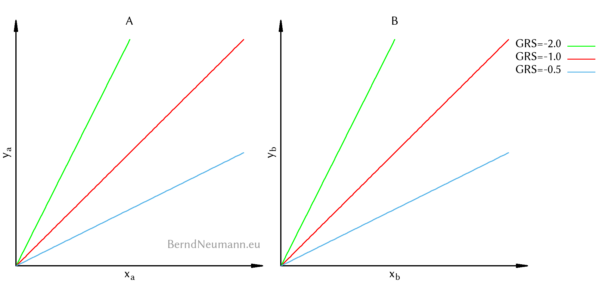
In both quantity of goods diagrams, all points with the same marginal rate of substitution are on a straight line through the origin and each line belongs to a certain \(\text{MRS}^x\). The corresponding equations are obtained by transforming the \(\text{MRS}^x\)-functions to \(y_a\) and \(y_b\) and taking the \(\text{MRS}^x\) as parameter. If we remember the three-dimensional representation of the \(\text{MRS}\) as a scalar field in Figure 3a, then these straight lines as iso-MRS lines
represent this scalar field just as the two-dimensional indifference curves represent the three-dimensional utility function. That the curves for the same \(\text{MRS}\) are straight lines is a property of the Cobb-Douglas preferences. The slope of the lines depends on the preferences and the \(\text{MRS}^x\). The more the individual prefers good \(Y\), the steeper the slope is and it is closer to the axis for good \(Y\). Likewise, the straight line is steeper for smaller, as absolute value larger, \(\text{MRS}^x\) and for larger, as absolute value smaller, \(\text{MRS}^x\) flatter and closer to the axis for good \(X\).
We arrive at the contract curve by combining the two goods quantity diagrams from Figure 4a into an Edgeworth box. Algebraically, this is done with the feasibility conditions. Together with the equation of the optimality condition we then have three equations with four variable quantities of goods. From these three we can derive the contract curve as one equation \(y_a(x_a)\). For this purpose, we geometrically rotate, following Figure 4a, the diagram of individual \(B\) by 180 degrees and shift it so that the Edgeworth box results. Possible bundles of goods are then exclusively valid allocations of the Edgeworth box and the optimality condition is fulfilled where lines of the same \(\text{MRS}^x\) or, according to Figure 4a, lines of the same color intersect. These intersections are the points of the contract curve.

point on the contract curve.
For the algebraic solution we put the feasibility conditions into the equation of the optimality condition: $$\begin{aligned} \frac{\alpha}{1-\alpha} \frac{y_a}{x_a} \; &= \; \frac{\beta}{1-\beta} \frac{(\omega^y-y_a)}{(\omega^x-x_a)} \end{aligned}$$
We solve this for \(y_a\) and obtain the set of Pareto efficient allocations as equation of the contract curve: $$\begin{aligned} y_a \; &= \; \frac{(1-\alpha)\beta \omega^y x_a}{\alpha\,(1-\beta)\,\omega^x \; - \; \alpha\,(1-\beta)\,x_a \; + \; (1-\alpha)\beta x_a} \end{aligned}$$
For this deduction, we have gone into the mathematical view in great detail, because otherwise the calculation procedure is slightly counter-intuitive: We usually draw the Edgeworth box first and then, as happened in Figure 3b, touching indifference curves, but we calculate in reverse order, first equating the marginal rates of the substitution and then limiting the allocations with the feasibility conditions to the Edgeworth box. This detailed exposition should have made clear that three steps are required to arrive at the contract curve, and each step corresponds to a distinct mathematical illustration and has its own economic meaning. One must
- determine the functions of the marginal rate of substitution;
- restrict the bundles of goods to those with the same marginal rate of substitution, i.e. equate the functions of the marginal rate of substitution;
- limit the bundles of goods to the feasible allocations of the Edgeworth box by using the feasibility condition and thereby express everything in the coordinate system in which one wants to draw the contract curve.
The order does not matter at all: You can also do the third step before the first one and therefore insert the feasibility conditions into the utility function of individual \(B\), but then you have to make the partial derivatives for the \(\text{MRS}^x_b\)-function a bit more complicated with the chain rule. The contract curve as result is the same in any case. – I want to point out another algebraic solution: One maximizes the utility of one individual under the three secondary conditions, the other individual had a certain utility level and both feasibility conditions were fulfilled. This maximization problem can be solved with the Lagrangian method. From the partial derivatives of the Lagrangian function we obtain a system of equations, which corresponds to the three steps just described. This method is geometrically clear and elegant, but also mathematically more demanding without improving the economic understanding. Therefore I will leave it at having briefly hinted at it.
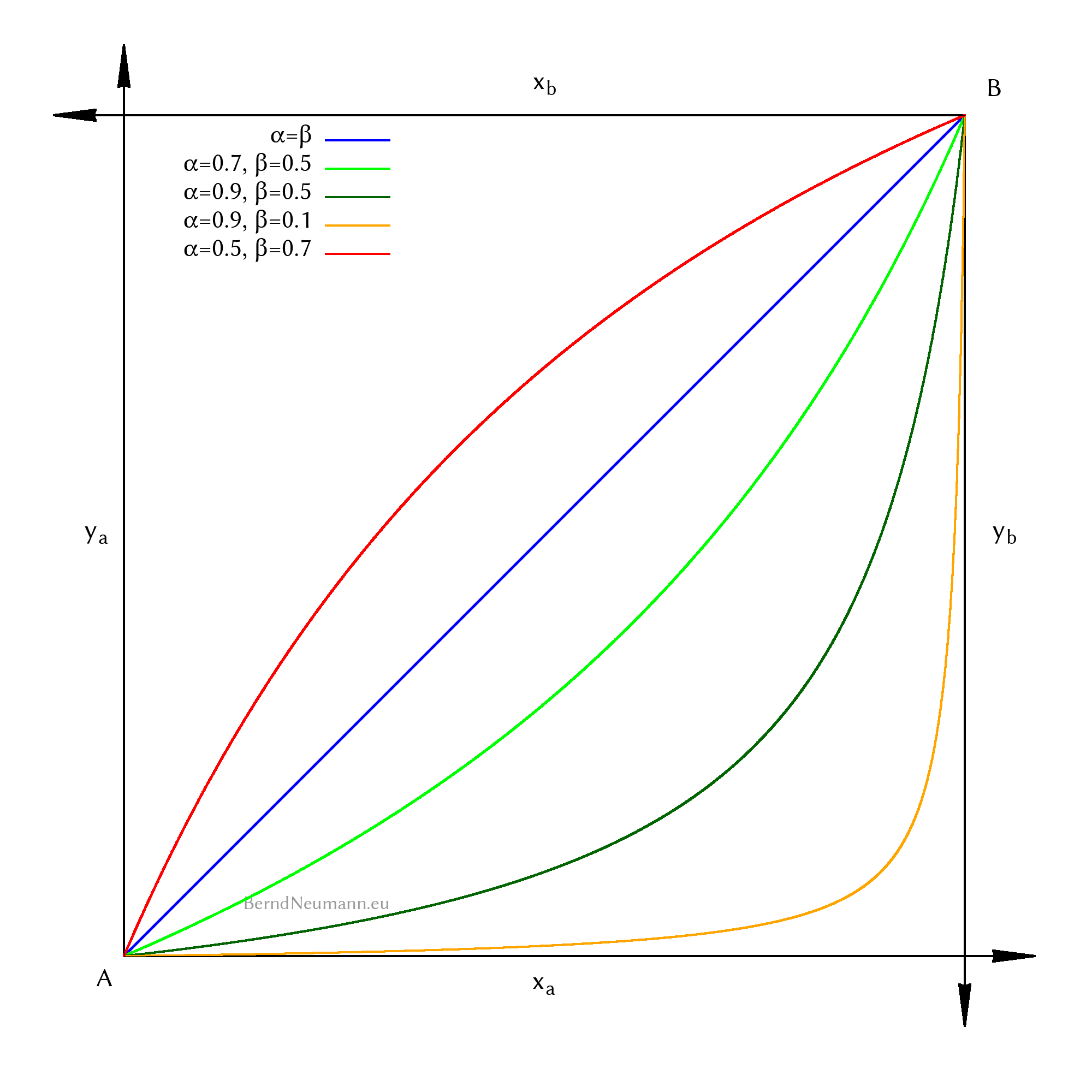
In the example calculations of the tutorials, a simple straight line equation usually emerges as a contract curve. This is the case if both individuals have the same preferences, i.e. if \(\alpha=\beta\) applies to our Cobb-Douglas utility functions. In the equation of the contract curve, then all \(\alpha\) and \(\beta\) are shortened and a straight line with the slope \(\frac{\omega^y}{\omega^x}\) remains. $$\begin{aligned} y_a \; &= \; \frac{\omega^y}{\omega^x}\;x_a \end{aligned}$$
Contract curves for different values of \(\alpha\) and \(\beta\) give a vivid impression:
Pareto efficient allocations as described by the contract curve are desirable states. Their derivation from the utility functions does not at all show that these states are reached. People trade on markets with quantities of goods and prices that did not occur at all in the derivation of the contract curve. For this reason, I emphasized above that the concepts of Pareto efficiency and market equilibrium must be considered separately. One should not be dissuaded from this, because bartering in the direction of a Pareto efficient allocation through the lenticular common better sets is obvious and seems rational. One must always keep in mind that here not two individuals exchange and one makes an offer to the other for mutual benefit. We are talking about markets where many individuals trade with quantities of goods and prices. So it remains clear that in deriving Pareto efficient allocations we were talking about what is desirable, but not about the result of market actions.
5. Individual Utility Maximization and Demand Functions
After the analysis of what is desirable, the question of the actual result of the acting arises: What happens if all individuals deal with the quantities of goods and prices in such a way that they maximize their personal benefit? – Let us calculate this for person \(A\) analogous to the maximization of utility in the partial analysis. Rather than by income, the secondary condition is determined by the initial endowment valued at \(p_x\) and \(p_y\): $$\begin{aligned} &\text{max}\;U_a(x_a, y_a)\\[1em] &SC: p_x x_a \; + \; p_y y_a \; \leq \; p_x \omega^x_a \; + \; p_y \omega^y_a \end{aligned}$$
Setting up the Lagrange function: $$ L(x_a, y_a, \lambda) \; = \; x_a^\alpha \, y_a^{(1-\alpha)} \, - \, \lambda \left( p_x \omega^x_a \; + \; p_y \omega^y_a \; - \; p_x x_a \; - \; p_y y_a \right) $$
The partial derivatives must equal zero: $$\begin{aligned} \frac{\partial L}{\partial x_a} \; &= \; \alpha \; x_a^{(\alpha-1)} \; y_a^{(1-\alpha)} \; + \; \lambda p_x \; = \; 0\\[1em] \frac{\partial L}{\partial y_a} \; &= \; x_a^\alpha \; (1-\alpha) \; y_a^{-\alpha} \; + \; \lambda p_y = \; 0\\[1em] \frac{\partial L}{\partial \lambda} \; &= \; p_x x_a \; + \; p_y y_a \; - \; p_x \omega^x_a \; - \; p_y \omega^y_a \; = \; 0 \end{aligned}$$
The solutions of this equation system are the Marshallian demand functions. To distinguish them from other quantities of goods, we mark them with an asterisk. It indicates that we are talking about a quantity of goods after utility maximization: $$\begin{aligned} x_a^*(p_x, p_y) \; &= \; \frac{\alpha\;(p_x \omega^x_a \; + \; p_y \omega^y_a)}{p_x}\\[1em] y_a^*(p_x, p_y) \; &= \; \frac{(1-\alpha)\;(p_x \omega^x_a \; + \; p_y \omega^y_a)}{p_y}\\[1em] \end{aligned}$$
Similarly, one gets the demand functions for Individual \(B\): $$\begin{aligned} x_b^*(p_x, p_y) \; &= \; \frac{\beta\;(p_x \omega^x_b \; + \; p_y \omega^y_b)}{p_x}\\[1em] y_b^*(p_x, p_y) \; &= \; \frac{(1-\beta)\;(p_x \omega^x_b \; + \; p_y \omega^y_b)}{p_y} \end{aligned}$$
There are three types of variables in Marshallian demand functions: Preferences in the form of the exponents \(\alpha\) and \(\beta\), initial endowments and prices. The first two come from the definition of the exchange economy (see above) and they are the minimum that has to be assumed as exogenously given. Therefore we treat them as constants. Prices, on the other hand, came into play due to budget constraints during utility maximization. They are variables, and therefore we write the Marshallian demand functions as a quantity of goods in dependence of the (variable) prices. We are talking about the utility maximizing behavior of individuals on the market and the question is: At what prices do we exchange? – Before we calculate this, let's dwell for a moment on the demand functions, since they can be used to clearly sketch the problem. This sketch will explain why we formulate the analysis of goods markets as a question of prices, and why prices are the answer to the question of a general equilibrium.
We have illustrated the Marshallian demand functions in partial equilibrium analysis in a price-quantity diagram. This does not help in the general equilibrium analysis with several goods. But we can draw the Marshallian demands for certain prices as points in the Edgeworth box by calculating the corresponding quantities of goods \(x^*\) and \(y^*\) for these prices. Such a demand point means that at the corresponding prices one wants to trade from the initial endowment to this bundle of goods, and can afford this bundle of goods at these prices. You can imagine it like this: We tell the individuals prices and then both point at the bundle of goods that they would like to have at these prices. They agree to trade when both point at the same allocation in the Edgeworth box.
Before we draw these demand points for different prices in the Edgeworth box, it is reasonable to calculate the exchange curve. It represents these demand points for all possible prices. To do this, we need to combine both demand functions of each person and eliminate the prices. We rearrange the Marshallian demand functions so that the prices are on one side as \(\frac{p_y}{p_x}\). For person \(A\) we get thereby: $$\begin{aligned} \frac{p_y}{p_x} \; &= \; \frac{x_a^* \; - \; \alpha \omega^x_a}{\alpha \omega^y_a}\\[1em] \frac{p_y}{p_x} \; &= \; \frac{(1-\alpha)\omega^x_a}{y_a^* \; - \; (1-\alpha) \omega^y_a} \end{aligned}$$
By equating and rearranging one obtains \(y_a^*(x_a^*)\): $$\begin{aligned} y_a^*(x_a^*) \; &= \; \frac{\alpha \omega^y_a(1-\alpha)\omega^x_a}{x_a^* \; - \; \alpha \omega^x_a} \; + \; (1-\alpha) \omega^y_a \end{aligned}$$
Similarly for Person \(B\) one obtains \(y_b^*(x_b^*)\): $$\begin{aligned} y_b^*(x_b^*) \; &= \; \frac{\beta \omega^y_b(1-\beta)\omega^x_b}{x_b^* \; - \; \beta \omega^x_b} \; + \; (1-\beta) \omega^y_b \end{aligned}$$
Let's look at the Edgeworth box and see how the points of Marshallian demand move across the exchange curve at different prices. This results in boundary solutions for high prices of a good. They are of no further interest here.

The exchange curves have two points of intersection. One is exactly on the initial endowment, because there are prices for both individuals at which they want to keep the initial endowment. However, this is the case for different prices, so that only one of them would like to keep the initial endowment, while the other would like to exchange goods. This intersection has no further meaning because the individuals point at different points in the Edgeworth box. This is not the case with the other intersection point. If the price line runs exactly through it, the points of Marshallian demand of both individuals are exactly on top of each other, both individuals point for these prices at the same allocation of the Edgeworth box. Only in this allocation and only for these prices we do have handshake, exchange and general equilibrium.
The mentioned sketch (see above) manifests itself in the question, how we will calculate this intersection and how we make sure, that it exists at all. Maybe the intersection point of the exchange curves in the graph is only accidental and does not exist at all for other preferences and initial endowments. To find out, we will assume that the Marshallian demand points are pointing at the same allocation of the Edgeworth box, and then look for prices that are consistent with this assumption. If we find prices that are consistent with this assumption, we have general equilibrium; if we do not find any, the theory of general equilibrium is reduced to saying that there is none at all.
With this sketch, the result of utility maximizing individual behavior on the market seems obvious, and the solution within reach. But there is still a pitfall lurking, which we will remove in the next section by first explaining the concept of excess demand
and thereby defining the market equilibrium. We then turn to the pitfall mentioned above and discuss the relativity of prices
in the context of Walras' law.
6. Walras' Law, Excess Demand and the Relativity of Prices
In the previous section, we described Marshallian demand points in such a way that we call out prices and the individuals point at the desired bundle of goods. Of interest is the point where both are pointing at the same allocation of the Edgeworth box. We now express this situation mathematically by looking at the quantities of goods offered and demanded: If one's Marshallian demand is greater than the initial endowment, one wants to buy more of this good; if it is smaller, one wants to sell a part of the initial endowment. This difference is called excess demand, and we will denote it with a \(\Delta\): $$\begin{aligned} \Delta x_a^*(p_x, p_y) \; &= \; x_a^*(p_x, p_y) \; - \; \omega^x_a\\[1em] \Delta y_a^*(p_x, p_y) \; &= \; y_a^*(p_x, p_y) \; - \; \omega^y_a\\[1em] \Delta x_b^*(p_x, p_y) \; &= \; x_b^*(p_x, p_y) \; - \; \omega^x_b\\[1em] \Delta y_b^*(p_x, p_y) \; &= \; y_b^*(p_x, p_y) \; - \; \omega^y_b \end{aligned}$$
The equations of excess demand describe how individuals act on the market. With them we can define the market equilibrium for a good. It occurs if the quantities offered and demanded for this good are equal, i.e. if the sum of excess demand is zero: $$\begin{aligned} \Delta x_a^* \; + \; \Delta x_b^* \; &= \; 0\\[1em] \Delta y_a^* \; + \; \Delta y_b^* \; &= \; 0 \end{aligned}$$
These equations mean that the Marshallian demands of both individuals point at the same allocation of the Edgeworth box. Writing the two equations for market equilibria not with excess demand but as the difference between Marshallian demand and initial endowment, we see that the equations for market equilibria correspond to the feasibility conditions. Market equilibrium thus means that individual consumption desires at the corresponding prices are consistent with the feasibility condition. In Figure 5 it is easy to see that the Marshallian demands do not take into account whether this consumption desire is consistent with the consumption desires of other individuals. The three statements that (1) Marshallian demands point at the same allocation, that (2) in all goods markets the quantity offered is equal to the quantity demanded, and that (3) Marshallian demands are consistent with the feasibility condition, describe the same fact. The equations for the market equilibria express it mathematically.
Given the equations for market equilibria, one might think that we only have to use the excess demand or demand functions and then see if we get the prices at which both goods markets are in balance. We have two equations and are looking for two prices. The solution seems trivial. However, there is still the mentioned pitfall in the way. For its solution, the concept of excess demand and the definition of market equilibrium are necessary.
For this we look back at the budget restrictions. On the one hand, it contains the value of the initial endowment, i.e. the quantities of goods multiplied by the prices; and it means that we can only afford bundles of goods whose value corresponds at most to the value of the initial endowment. The bundle of goods that one would like to afford according to one's Marshallian demand has always the same value as the initial endowment, for no one is satisfied with getting less in an exchange than he has given. In the geometric view, we see this in the fact that the Marshallian demand points are on the budget line, except for the boundary solutions. This is not only true for certain prices or under certain conditions, but it is true per definition of Marshallian demands as a bundle of goods with maximum utility. Its value is therefore not only equal to the value of the initial endowment, but identical with it: $$\begin{aligned} p_x\,x_a^* \,+\, p_y\,y_a^* \; &\equiv \; p_x\,\omega^x_a \,+\, p_y\,\omega^y_a\\[1em] p_x\,x_b^* \,+\, p_y\,y_b^* \; &\equiv \; p_x\,\omega^x_b \,+\, p_y\,\omega^y_b \end{aligned}$$
We rearrange by bracketing out the prices and write the differences in the brackets as excess demand: $$\begin{aligned} p_x \, \Delta x_a^* \;+\; p_y \, \Delta y_a^* \; &\equiv \; 0\\[1em] p_x \, \Delta x_b^* \;+\; p_y \, \Delta y_b^* \; &\equiv \; 0 \end{aligned}$$
These two identities state that the value of the sum of the excess demand of each person is identical to zero. It follows that the value of excess demand aggregated over individuals is also identical to zero. We add the equations and bracket out the prices: $$\begin{aligned} p_x\,(\Delta x_a^* + \Delta x_b^*) \;+\;p_y\,(\Delta y_a^* + \Delta y_b^*) \; \equiv \; & 0 \end{aligned}$$
This identity is Walras' law. – Let's see what follows from this for the equilibrium prices: In Walras' law we have the aggregated excess demand of each market, and we had defined as market equilibrium that they equal zero. Suppose the market for good \(X\) is in equilibrium, so that $$\begin{aligned} \Delta x_a^* \; + \; \Delta x_b^* \; &= \; 0 \end{aligned}$$ Further we know that the prices \(p_x\) and \(p_y\) are both greater than zero. It follows from Walras' law that $$\begin{aligned} \Delta y_a^* \; + \; \Delta y_b^* \; &= \; 0 \end{aligned}$$ So if one market is in equilibrium, it follows that the other market is also in equilibrium. If you generalize to any number of goods, you will see that all goods markets are in equilibrium if all but one of them are in equilibrium.
This reveals what the pitfall is. Above we had defined the market equilibrium for both (two) goods markets and intuitively thought: With two equations we get a unique solution for two (unknown) prices. Now it turned out that one of the equations follows from the other. Therefore we have only one equation for two unknown prices. You can this in figure 5 by the fact that it depends on the slope of the budget line. This slope is \(-\frac{p_y}{p_x}\). So we are looking for a price ratio, because the prices are only determined up to one price. Therefore we can set the price of a good as a so-called Numéraire equal to one and understand all other prices as relative prices in relation to this good. For our two-goods case, however, we will leave the fraction as it is.
At this point the representation of the exchange economy with only two goods reaches its limits. Walras' law says that we have an equilibrium in all goods markets if we have an equilibrium in all but one market. In an economy with only two goods all but one
is only one. The dazzling point of the general equilibrium, to have a market equilibrium on many interdependent markets at the same time, might thereby fade away. One could drink until this circumstance appears beautiful with the argument, good \(X\) or \(Y\) is not a single good, but a combination of goods. This argument is true. But no matter how you think about this, it is important to know, that the principle is the same for two goods markets, where one goods market represents all but one
, and both goods markets represent many (all) markets
.
7. The General Equilibrium
We now know that in this two-goods case we obtain the equilibrium prices or their quotients by formulating the equilibrium condition for only one goods market. We choose good \(X\): $$\begin{aligned} \Delta x_a^* \; + \; \Delta x_b^* \; &= \; 0\\[1em] (x_a^* \;-\; \omega^x_a) \; + \; (x_b^* \; -\; \omega^x_b) \; &= \; 0 \end{aligned}$$
We use the Marshallian demand functions, which we have calculated further above. We add an asterisk to the prices to indicate that they are equilibrium prices: $$\begin{aligned} \frac{\alpha\;(p_x^* \omega^x_a \; + \; p_y^* \omega^y_a)}{p_x^*} \;-\; \omega^x_a \; + \; \frac{\beta\;(p_x^* \omega^x_b \; + \; p_y^* \omega^y_b)}{p_x^*} \,-\,\omega^x_b\ \; &= \; 0 \end{aligned}$$
This equation we solve for the quotient of the prices and obtain: $$\begin{aligned} \frac{p_y^*}{p_x^*} \; &= \; \frac{(1-\alpha)\omega^x_a+(1-\beta)\omega^x_b}{\alpha\omega^y_a + \beta\omega^y_b} \end{aligned}$$
In this equation, prices are determined by the exponents of the utility functions and the initial endowments, i.e. exclusively by variables that define this exchange economy. We obtain prices for all possible exponents and initial endowments, because both numerator and denominator of the equation are always positive numbers. It cannot happen that the prices would not be defined because the denominator would result in zero.
The prices \(p_x^*\) and \(p_y^*\) describe an equilibrium on the market for good \(X\), and this is an equilibrium on all goods markets except one. According to Walras' law, all goods markets are thus in equilibrium at these prices. This shows that a general equilibrium exists for all valid exponents of utility functions and all valid initial endowments: $$\begin{aligned} \Delta x_a^*(p_x^*, p_y^*) \; + \; \Delta x_b^*(p_x^*, p_y^*) \; &= \; 0\\[1em] \Delta y_a^*(p_x^*, p_y^*) \; + \; \Delta y_b^*(p_x^*, p_y^*) \; &= \; 0 \end{aligned}$$
The general equilibrium is also called Walrasian equilibrium or competitive equilibrium. The two equations describe it by means of excess demand with respect to the markets for good \(X\) and good \(Y\). Hal Varian (1987: p. 592) also describes it in this way. Andreu Mas-Colell (1995: p. 519) offers an interesting alternative by describing the Walrasian equilibrium from the perspective of individuals. For this purpose, he defines all bundles of goods \((x_i^{'}; y_i^{'})\) that the individual \(i\) can afford at the prices \((p_x^*; p_y^*)\) with a price-dependent budget set \(\mathbb{B}(p_x^*; p_y^*)\). A Walrasian equilibrium exists if all individuals realize the best bundle of goods \((x_i^*; y_i^*)\) they can afford at the prices \((p_x^*; p_y^*)\): $$\begin{aligned} U(x_i^*; y_i^*) \geq U(x_i^{'}; y_i^{'}) \qquad \forall\;\;(x_i^{'}; y_i^{'})\in\mathbb{B}(p_x^*; p_y^*) \end{aligned}$$
The described fact is the same, only that in this case both the formulation with words and the equations are different. That both formulations are equivalent can be easily understood: If everyone realizes the best bundle of goods that he can afford at these prices, then he must be able to exchange it for his initial endowment. For this purpose he must be able to exchange his excess demand on the market for each good, i.e. the excess demands of all individuals must be compatible with each other, so that the sum of all excess demands for each good must be zero. – Since both formulations are equivalent, they describe the same prices. By the different formulations of the Walrasian equilibrium it becomes clear why it is said that a Walrasian equilibrium is just this price vector. Because prices are essential for the Walrasian equilibrium and not how the definition is formulated in detail.
We have calculated this price vector in this exchange economy for all valid utility functions and initial endowments, thus demonstrating the existence of general equilibrium. This says the essential. For the sake of completeness, we calculate the quantities of goods in equilibrium by inserting the equilibrium prices into the Marshallian demand functions. We mark these quantities of goods with a second asterisk to indicate that the quantities of goods are maximum utility quantities at equilibrium prices: $$\begin{aligned} x_a^{**} \; &= \; x_a^*\,(p_x^*, p_y^*)\\[1em] y_a^{**} \; &= \; y_a^*\,(p_x^*, p_y^*) \end{aligned}$$
The prices disappear from the equations and we get an equilibrium allocation that depends only on initial endowments and preferences: $$\begin{aligned} x_a^{**} \; &= \; \alpha \omega^x_a \; + \; \frac{\alpha (1-\alpha)\omega^x_a\omega^y_a+\alpha (1-\beta)\omega^x_b\omega^y_a}{\alpha\omega^y_a + \beta\omega^y_b}\\[1em] y_a^{**} \; &= \; (1-\alpha)\omega^y_a \; + \; \frac{\alpha(1-\alpha)\omega^y_a\omega^x_a+(1-\alpha)\beta\omega^y_b\omega^x_a}{{(1-\alpha)\omega^x_a+(1-\beta)\omega^x_b}} \end{aligned}$$
The corresponding quantities for person \(B\) can be calculated in the same way. But you can also make it simple and use the feasibility condition: $$\begin{aligned} x_b^{**} \; &= \; \omega^x_a \,+\, \omega^x_b \,-\, x_a^{**}\\[1em] y_b^{**} \; &= \; \omega^y_a \,+\, \omega^y_b \,-\, y_a^{**} \end{aligned}$$
This equilibrium is the result of market activity, which we contrasted with what is desirable at the very beginning (see above). All equations now depend only on preferences and initial endowments. The following illustration shows how the equilibrium point moves if preferences or initial endowments change:

8. The Justification of Market Equilibrium
We neglected one small thing while calculating the general equilibrium. Although the equilibrium prices guarantee that a general equilibrium is possible, they do not justify that it is realized. The Walrasian equilibrium, like everything in microeconomics, is based on the justification scheme of individual utility maximization. It stood at the beginning of the calculation (see above) and is inherent in all equations in the form of the (utility maximizing) Marshallian demand. In Marshallian demand functions, individuals are price takers: they vary the quantities of goods offered and demanded for given prices. This is a problem if we also try to explain the adjustment of prices as individual utility maximization. After all, who should initiate changes in prices if all individuals consider themselves as price takers (see Varian 1978: Ch. 21.4, p. 398)? We have a problem of justification.
The reason for this problem of justification is that the theory of general equilibrium belongs to comparative statics, whereas the question of the Tâtonnement process, i.e. the process of approaching
at equilibrium, requires a dynamic analysis. Metaphorically speaking, we have the finish photo of a 10-kilometer run, and we find that this photo cannot answer the legitimate and meaningful question of how the race went. There will therefore be no elegant equation to answer this justification problem. The question is how to deal with it, and the answer is one of personal taste.
Andreu Mas-Colell strictly separates the static analysis from the dynamic one. To define the equilibrium of a market, he briefly notes: At a market equilibrium where consumers take prices as given, markets should clear.
(Mas-Colell 1995: Sec. 15.B, p. 518) Only the subjunctive quietly indicates that there might be a problem. The dynamic analysis has its place for Mas-Colell in a later chapter (Mas-Colell 1995: Sec 17.H, p. 620 ff). The advantage is that this avoids asking questions of dynamics to the static analysis that it cannot answer at all. The disadvantage is that one ignores an obvious question just as strictly as one has separated statics and dynamics.
Somewhat more justification can be read implicitly from Walras's concept of economics as a science. Science, according to Walras, is dependent on abstracting from reality (Walras 1874: Sec. 30, p. 27 f); and on real markets we see that they tend to equilibrium by themselves (Walras 1874: Sec. 61, p. 66 f). This would provide an empirical basis for the idealized equations of market equilibria. The advantage is that one addresses the reference to real markets. The disadvantage is that an empirical argument is theoretically not convincing. One does not answer the question of why the stone falls to the ground with gravity, but with the statement that in the end it always lies on the ground.
Hal Varian takes the most popular approach through a Walrasian auctioneer. One should imagine an auctioneer announcing prices on all markets, whereupon the market participants, according to their Marshallian demand functions, state the amounts of goods they offer and demand at these prices. The auctioneer adjusts the price until the supply equals the demand and only at this price the exchange actually takes place. (cf. Varian 1978: p. 398 and 1987: p. 588) Varian is aware that Walras himself never meant it this way with that auctioneer. Although Walras hints at this idea in the preface (Walras 1874: Preface, p. ix), he does not think of an imaginary auctioneer that must be imagined in all markets, but cites such well-organized markets as a vivid example of competition (cf. Walras 1874: Sec. 41, p. 42 f). Varian therefore very aptly calls Walrasian auctioneer an elaborate mythology
(Varian 1978: 398), which is intended to solve the paradox that price takers must adjust prices.
The advantage of the Walrasian auctioneer is to provide a brief and vivid explanation of the paradox in question, in which individuals act consistently with Marshallian demand functions as price takers. The serious disadvantage is, besides the fact that something is foisted on Walras that he never said, that we want to talk about free markets and should imagine an imaginary price dictator who enforces the required market equilibrium.
I would like to suggest another way. The starting point is to clearly state that a model of comparative statics cannot explain the process of equilibrium. If one wants to at least make it plausible without opening a new chapter in microeconomics, one must interpret the term price taker
somewhat more freely by saying that a seller cannot sell more expensively than the others, but can sell more cheaply. Let us look at the seller of a good for which the price is higher than in Walrasian equilibrium. He starts the trade with his initial endowment and trades piece by piece along the price line towards his Marshallian demand point. But before he reaches it, he can no longer find buyers who want to buy at this high price. The seller cannot realize his utility maximizing bundle of goods, so that the indifference curve of the realized bundle of goods intersects with the price line instead of just touching it. Thus there must be an overlap of his better set and possibilities set. If he would lower the price slightly now and sell more, he can realize a bundle of goods in this intersection set and thus be better off. The lowering of prices is therefore rational for this seller. The same applies to all salesmen of this good until the price has fallen to that of the Walrasian equilibrium.
The essential advantage of this explanation is to justify with individual utility maximization as originally thought by Walras (Walras 1874: Lesson 8, p. 77 ff), and there is no need to open a new chapter in microeconomics. However, these great advantages are countered by equally serious disadvantages: The reinterpretation of the term price taker
seems minor, but is not consistent with the price taker in the sense of Marshallian demand. The explanation is inconsistent. It also suggests that it is a mathematical and thus well-founded model, but is rather a plausible scribble in the existing diagrams. With this explanation the advantages and disadvantages are the largest. After careful consideration, I think that with this explanation, the bottom line is that the lesser evil is chosen.
Three aspects should be noted: 1. the theory of general equilibrium is comparative statics, and it cannot explain the formation of the market equilibrium assumed by definition. 2. the Walrasian equilibrium is nevertheless not a castle in the air made of mathematical equilibrium fantasies. Various heuristic explanations make the establishment of the equilibrium plausible. None of them is flawless, but for plausibility it should be enough. If you want to know more, you have to be referred to the dynamic equilibrium analysis of the Tâtonnement process. 3. the question of the establishment of equilibrium vividly demonstrates that the theory of general equilibrium depends on the perfect competition of many individuals. We will take up this aspect again in the digression on Edgeworth's criticism.
9. The First Theorem of Welfare Economics
First, we used the marginal rate of substitution to explain the concept of Pareto efficiency (see above) to show which allocations in the Edgeworth box are desirable. We have shown the set of these allocations as the contract curve (see above). We then calculated which allocation is realized when individuals, each on their own and in perfect competition with each other, maximize their utility (see above). This resulted in the allocation of the general equilibrium (see above). Now we will examine the relationship between the allocation of general equilibrium and the desirable Pareto efficient allocations.
With intuitive arguments, this can be done very quickly: We know from partial equilibrium analysis that the marginal rate of substitution is equal to the price ratio when an individual reaches his maximum utility. In general equilibrium each individual reaches his maximum utility at the prevailing equilibrium prices. Since these prices are the same for all, the marginal rate of substitution must be the same for all individuals as well. Therefore, the allocation of the general equilibrium as it is achieved under perfect competition must be a Pareto efficient allocation. In other words: Through free markets and perfect competition we always achieve a desirable allocation, at least with respect to Pareto efficiency. Every Walrasian equilibrium is Pareto efficient. This is the First Theorem of Welfare Economics.
Let us look at this in the language of equations by calculating for both individuals what marginal rate of substitution they have in the allocation of the general equilibrium: $$\begin{aligned} \text{MRS}_a^x\Big(x_a^{**}, y_a^{**}\Big) \; &= \; \text{MRS}_a^x\Big(x_a^*(p_x^*, p_y^*), y_a^*(p_x^*, p_y^*)\Big)\\[1em] \text{MRS}_b^x\Big(x_b^{**}, y_b^{**}\Big) \; &= \; \text{MRS}_b^x\Big(x_b^*(p_x^*, p_y^*), y_b^*(p_x^*, p_y^*)\Big) \end{aligned}$$
On the right side of both equations we use the function of the marginal rate of substitution as we derived it further above: $$\begin{aligned} \text{MRS}_a^x\Big(x_a^{**}, y_a^{**}\Big) \; &= \; - \; \frac{\alpha}{1-\alpha} \; \frac{y_a^*(p_x^*, p_y^*)}{x_a^*(p_x^*, p_y^*)}\\[1em] \text{MRS}_b^x\Big(x_b^{**}, y_b^{**}\Big) \; &= \; - \; \frac{\beta}{1-\beta} \; \frac{y_b^*(p_x^*, p_y^*)}{x_b^*(p_x^*, p_y^*)} \end{aligned}$$
We use the Marshallian demand functions that we derived by the utility maximization of the individuals (see above): $$\begin{aligned} \text{MRS}_a^x\Big(x_a^{**}, y_a^{**}\Big) \; &= \; - \; \frac{\alpha}{1-\alpha} \; \frac{\frac{(1-\alpha)\;(p_x^* \omega^x_a \; + \; p_y^* \omega^y_a)}{p_y^*}}{\frac{\alpha\;(p_x^* \omega^x_a \; + \; p_y^* \omega^y_a)}{p_x^*}} \\[1em] \text{MRS}_b^x\Big(x_b^{**}, y_b^{**}\Big) \; &= \; - \; \frac{\beta}{1-\beta} \; \frac{\frac{(1-\beta)\;(p_x^* \omega^x_b \; + \; p_y^* \omega^y_b)}{p_y^*}}{\frac{\beta\;(p_x^* \omega^x_b \; + \; p_y^* \omega^y_b)}{p_x^*}} \end{aligned}$$
By reducing, one obtains that both marginal rates of substitution are equal to the negative ratio of the equilibrium prices: $$\begin{aligned} \text{MRS}_a^x\Big(x_a^{**}, y_a^{**}\Big) \; &= \; - \; \frac{p_x^*}{p_y^*} \\[1em] \text{MRS}_b^x\Big(x_b^{**}, y_b^{**}\Big) \; &= \; - \; \frac{p_x^*}{p_y^*} \end{aligned}$$
Thus, the marginal rate of substitution of individual \(A\) equals the marginal rate of substitution of individual \(B\), and the allocation of the general equilibrium with the consumed quantities of goods \(x_a^{**}\), \(y_a^{**}\), \(x_b^{**}\), \(y_b^{**}\) is a Pareto efficient allocation. $$\begin{aligned} \text{MRS}_a^x\Big(x_a^{**}, y_a^{**}\Big) \; &= \; \text{MRS}_b^x\Big(x_b^{**}, y_b^{**}\Big) \end{aligned}$$
Finally, the following graphic illustrates this relationship in the Edgeworth box. But in order that one can see in these pictures the persuasive power of mathematical clarity in the sense of Walras (1874: Lesson 3, Section 30) or even an aesthetic of the Méchanique Sociale
following the example of the Méchanique Celeste
(Edgeworth 1881: 12), it should be remembered that the Pareto efficient allocations of the contract curve were achieved in a completely different way than the Walrasian equilibrium – and yet the Walrasian equilibrium for different preferences and initial endowments is exactly on the contract curve.

10. Digression: Edgeworth and the Perfection of the Markets
We have shown by mathematical means that free markets are efficient. Although we calculated with a two-goods two-person exchange economy and illustrated it in the Edgeworth box, we actually meant perfect markets with many market participants. Hal Varian offers the explanation that the two individuals represent the average preferences of two different types of consumers (Varian 1987: 588), and Andreu Mas-Colell points out that it is a matter of presenting the principle in the simplest possible way (Mas-Colell 1995: 516, 526). Both are true, and mathematically it is no magic trick to extend the representation to any number of individuals and goods. But this only works algebraically and you have to do it without the vividness of an Edgeworth box.
However, the presentation in the Edgeworth box should not make us forget that we have assumed perfect markets and it is more important to critically reflect on this assumption than to justify the presentation in the Edgeworth box alone. Such criticism does not necessarily mean that the assumption is wrong and the mathematics of pure economics is hocus-pocus. On the contrary: mathematics is a sharp analytical instrument with which a sophisticated theory was developed within a surprisingly short time in the course of the Neoclassical period. The strength of mathematics occasionally is to precisely name an assumption such as the perfection of markets and thereby make it accessible to a targeted criticism in the first place.
Marie-Esprit Léon Walras published the Éléments d'Économie Politique Pure ou Théorie de la Richesse Sociale
in 1874, and thereby presented a first draft of the mathematically formulated general equilibrium, which Francis Ysidro Edgeworth criticized with detailed mathematical considerations only a few years later in Mathematical Psychics
(1881). His criticism aimes at the assumption of perfect markets, and he presents four structural imperfections. Here is just one example: The labor market does not consist of many individual offerers and demanders of labor, but of a union representative and a representative of the employers, so that despite the large number of individuals involved, this market behaves like a negotiation between only two parties (cf. Edgeworth 1881: 44f, 49).
This goes far beyond the lapidary statement that reality never corresponds exactly to the idealized model with which it is explained. Edgeworth thinks of a completely different model. – Walras compared the assumption of perfect markets with the assumption of frictionless transmission of force in mechanics (Walras 1874: no. 41); and also Varian (1978: 216) uses this metaphor to justify. The idea is that the functioning of markets is represented by perfect competition in pure form
, and that by mathematically studying this ideal type one recognizes the essence of the market without making the theory unnecessarily complicated by frictional losses arising in reality. Edgeworth, on the other hand, believes that this idealization does not sufficiently capture the essence of the market. Instead, he draws the picture of a continuum, with the case of perfect competition at one end and the negotiation of two people at the other. One consequence of this is that the unambiguous definiteness of the equilibrium allocation, which seems mechanical and like a law of nature
, as we have seen it in figure 7 and figure 9, is dropped (Edgeworth 1881: page 46). The equilibrium allocation is only more or less determined depending on the extent of the imperfection of a market. In the case of negotiation between two persons, one can only say that they will agree on some point of the contract curve within the common better set (here best seen in Figure 3b). The unambiguity of the Walrasian equilibrium is replaced by what is now known as the Edgeworth theorem: (\(\alpha\)) Contract without competition is indeterminate, (\(\beta\)) Contract with perfect competition is perfectly determinate, (\(\gamma\)) Contract with more or less perfect competition is less or more indeterminate.
(Edgeworth 1881: 20.)
At first glance, this criticism seems to call into question everything that has been said so far. Edgeworth criticizes the assumption that is tacitly accompanying the model from the beginning and up to the First Theorem of Welfare Economics. He is well aware of the scope of his criticism and at one passage about the imperfection through monopoly positions he hints to go not without trembling
(Edgeworth 1881: page 47.) beyond Cournot's theory of monopoly. This weighs all the more heavily because Edgeworth believes that markets will tend to become increasingly imperfect over time (Edgeworth 1881: p. 50). But Edgeworth does not want to make such a fundamental critique. The assumption of perfect competition and the associated equilibrium mathematics is justified, and Edgeworth has nothing but praise for his colleagues William Stanley Jevons, Alfred Marshall and Léon Walras.
Edgeworth' punch line is another: Walrasian equilibrium, as we have derived it further above, is unambiguously determined by preferences and initial endowment, and Walras believed that the price in equilibrium expresses the true value of goods. This value is a natural fact
(Walras 1874: Section 28) and equilibrium has the character of a natural law independent of human will. The value is not subject to human decision-making (Walras 1881: Section 23-26), so that the allocation of the equilibrium, i.e. the resulting distribution of goods, is not an ethical question. Edgeworth opposes this separation of economics and ethics. For his argumentation he was the first to develop the concept of the contract curve, and for him it is clear, even without the First Theorem of Welfare Economics, that rational individuals always achieve an allocation of the contract curve within the common better set because both parties have an interest in it (Edgeworth 1881: 29, 54). But the interests of the parties are irreconcilable in the question of which allocation of the contract curve they realize, because there every gain of one is the loss of the other. This opposition of interests was the characteristic evil of imperfect markets, and that is what Edgeworth was concerned with the concept of the contract curve. The opposition leads to deadlock
and motivates hypocrisy and the objectionable arts of higgling
(Edgeworth 1881: 29f).
According to Edgeworth, only an ethical principle of arbitration (Edgeworth 1881: 51) could overcome this opposition of interests, so that the idea of competition had to be supplemented by ethical considerations. Edgeworth counters the separation of ethics from economics, understood in terms of natural science and mechanics, by arguing that economic thinking inevitably leads to ethical thinking (Edgeworth 1881: 56). This is the astonishing conclusion that Edgeworth derives from the critique of the assumed perfection of markets. We should keep it in mind when we talk today about the contract curve, Walrasian equilibrium and the First Theorem of Welfare Economics.
11. Final Remarks
The aim of this article is to present the basic features of the theory of general equilibrium up to the First Theorem of Welfare Economics in an exchange economy in such a way that mathematics is not only geometrically vivid, but also clear in its economic meaning and that the mathematical nature of economic thinking becomes tangible, so that some students of economics can not only solve an exam question after this tutorial
, but can independently apply the model of the exchange economy. If this is successful, my expectations associated with this article are completely fulfilled.
Furthermore, I would be glad if the last part made clear that the critical examination of economics is an exciting issue. Even if in economics one feels less like doing critical reflection than elsewhere, Edgeworth may have made it clear that such reflections can broaden the understanding of economics and need not necessarily be blueprints for Politburo propaganda sessions.
The critical excursion to Edgeworth is also connected with the hope of having sparked curiosity in some readers about the texts of the classics. Although the study of economics is largely a textbook study of the state of the art
, reading the classics offers more than the puzzle pieces that have found their way into the canon of textbooks. As we were able to see impressively from Edgeworth, this applies especially to the question of the relationship between economics and ethics. In times of climate change and increasing economic crises, economists should have more to say than just recommend internalizing external effects. Wise is therefore the advice that Jevons (1871) gives at the end of his introductory chapter: We can study economics away from moral considerations, but if time permits, no one forbids us to grow alongside value-free economics a second blade of grass in the form of ethical studies.
References
Edgeworth, Fancis Ysidro (1881): Mathematical Psychics. An Essay on the Application of Mathematics to the Moral Sciences. London. Online in the McMaster University Archive for the History of Economic Thought.
Jevons, William Stanley (1871): The Theory of Political Economy. 5th Edition, New York 1965.
Mas-Colell, Andreu; Whinston, Michael D.; Green, Jerry R. (1995): Microeconomic Theory. New York, Oxford.
Varian, Hal Ronald (1987): Intermediate Microeconomics. A Modern Approach. 8th Edition, 2010. New York, London.
Varian, Hal Ronald (1978): Microeconomic Analysis. 3rd Edition 1992. New York, London.
Walras, Marie-Esprit-Léon (1874): Elements of Theoretical Economics or the Theory of Social Wealth. Translation of the 3rd Edition (1896) by Donald A. Walker and Jan van Daal. Cambridge University Press 2014.
Bernd Neumann,