Contents

1. The Rationality of the Individual

2. The Indifference Curve

3. The Utility Function

4. The Budget Constraint

5. The Maximization of Utility

6. The Lagrangian Method

7. The Edgeworth Box

8. Final Remark

1. The Rationality of the Individual

Microeconomics explains economics from the point of view of the single individual, thus following the paradigm of Methodological Individualism (Wikipedia: Methodological Individualism). The first related assumption is that individuals act rationally. In the terminology of economics, they maximize their utility, which means striving for the greatest possible happiness or well-being. One often speaks of the human being as an egoistic utility maximizer. But this is misleading, because it suggests that economics declare the morally questionable quality of egoism to be its anthropological model, and egoism even to be a morally desirable or at least a morally legitimate quality. This is incorrect, because microeconomics is a model of human behavior in the sphere of economy, and this model claims nothing more than to explain economy. An ethical theory or philosophical anthropology is thus not claimed. One can imagine it that way: If someone invites his friends to a barbecue because of his sociable and generous nature, he does not become a morally questionable egoist, because he wants to save some money and therefore buys the crate of beer and the barbecue coal in the supermarket, which has both on special offer. – Untouched by this sometimes misunderstood image of man, it remains that economics also has to do with ethical questions. Within a digression in the article on exchange economy (Digression: Edgeworth and the Perfection of Markets) I will come back to this.

Utility-maximizing rationality cooks on a different flame than an ethical or anthropological theory: If someone likes chocolate ice cream more than vanilla ice cream, and we offer him to choose either a ball of chocolate or a ball of vanilla, then utility-maximizing rationality means that with the ball of chocolate ice cream he chooses the option he prefers. It would be irrational to choose the less favored option when he could have chosen better.

In the model of microeconomics we study the choice between bundles of goods. This is the combination of at least two goods, each in a certain quantity. We usually limit ourselves to two goods, because the two-dimensional case can be well illustrated with drawings. A bundle of goods is usually written as a tuple by writing the contained quantities of goods in round brackets. When choosing between the two balls of ice cream, the bundle of goods consisting of one ball of chocolate and zero balls of vanilla \((1; 0)\) was preferred to the bundle of zero balls of chocolate and one ball of vanilla \((0; 1)\). If you offer one ball of chocolate \((1; 0)\) or two balls of vanilla \((0; 2)\), vanilla could be the bundle of choice. There is nothing irrational about this, because we are not looking at the choice between chocolate and vanilla, but at the choice between bundles of goods.

The utility maximizing decision for a certain bundle of goods consists of two parts: On the one hand, we use the preferences in the form of a utility function to describe for each conceivable bundle of goods which other bundles of goods are better, which are worse and which are equally good. On the other hand, we use the budget restriction to describe which bundles of goods are achievable because they can be afforded. These are the bundles of goods of the budget set or possibility set. Utility maximization means to combine both parts by calculating, which bundle of goods of the possibility set is preferred to all other bundles contained in it and thus is chosen as the utility maximizing bundle of goods. The structure of the following sections is based on this division. We start with the preferences.

2. The Indifference Curve

I mentioned that you usually restrict yourself to two goods, because that is enough to explain the principle and you can illustrate the two goods case in diagrams. We will do the same and call the goods \(X\) and \(Y\). The quantity of good \(X\) is called \(x\), the quantity of good \(Y\) is called \(y\), and a bundle of goods is called \((x; y)\). Let us draw a diagram of quantities of goods, in which we plot the quantity of good \(x\) on one axis and the quantity of good \(y\) on the other axis. The points of this diagram represent every imaginable bundle of goods.

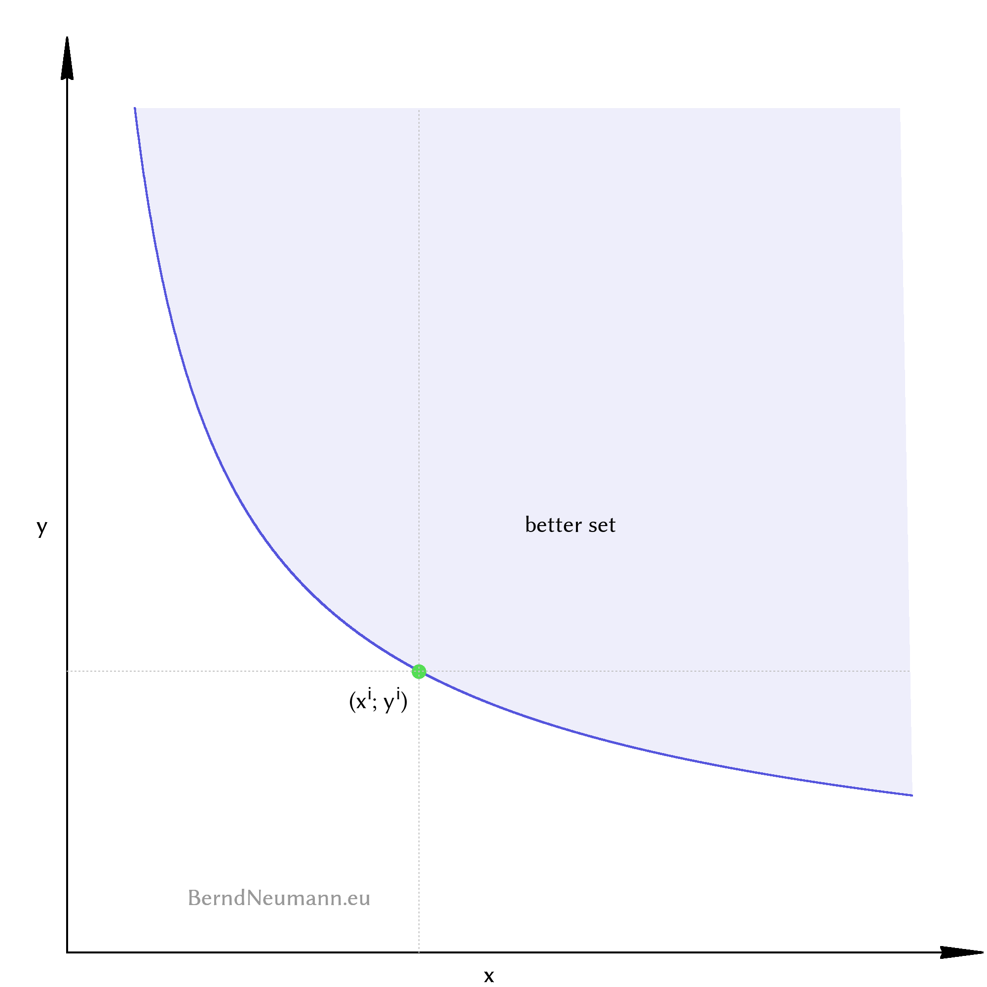
In this diagram we draw a bundle of goods \((x^{i}; y^{i})\) and ask: How does the consumer valuate this bundle of goods in terms of utility compared to other bundles of goods? Which bundle of goods does the consumer prefer to the bundle \((x^{i}; y^{i})\), which does he find worse and which just as good? – Assuming non-saturation means that a bundle of goods is always preferred if it contains more of at least one good and not less of any other. In Figure 1 these are all bundles that are located right above \((x^{i}; y^{i})\). Correspondingly, the consumer considers all bundles of goods which are on the left below \((x^{i}; y^{i})\) to be worse. The bundles of goods that are as good as \((x^{i}; y^{i})\) must lie on a curve that runs from \((x^{i}; y^{i})\) to the upper left and lower right. This curve of bundles of goods of the same utility level is called indifference curve. The individual does not care which of these bundles of goods he has, because the associated welfare is the same. All bundles of goods that lie above an indifference curve are preferred to bundles of goods of the indifference curve. They form the better set for all bundles of this indifference curve.

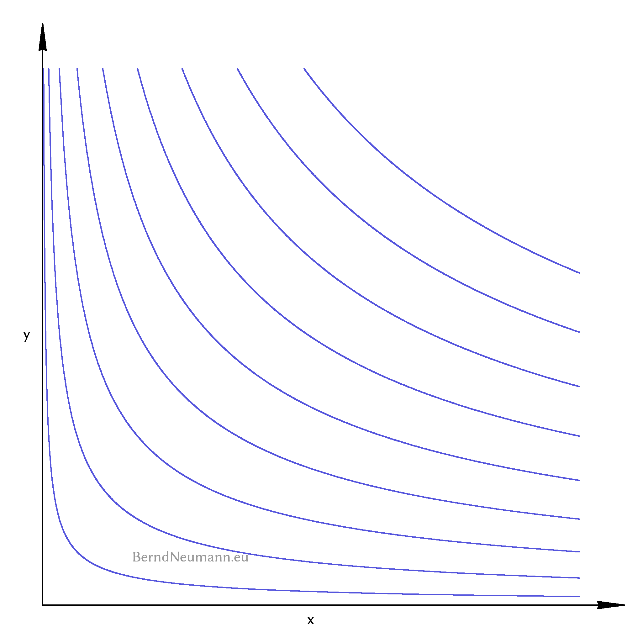
Indifference curves cannot intersect. If indifference curves would intersect, the bundles of goods of the one indifference curve would be partly better, at one point equally good and partly worse than the bundles of the other indifference curve. That would be irrational. There are infinitely many indifference curves that are infinitely close to each other, but they never intersect. Let's draw some indifference curves to get an idea of what they look like.

3. The Utility Function

Our goal is to decide for any two bundles of goods which one the consumer considers to be better and which one he considers to be equally good. Figure 2 takes us closer to this by numbering all indifference curves from bottom left to top right with a steadily increasing number. If we can then decide about two bundles of goods which numbers their respective indifference curves have, it is clear which one is preferred. This numbering is provided by a utility function which assigns a number to each bundle of goods. Bundles of goods with the same number lie on the same indifference curve, bundles of goods with a higher number lie on a higher indifference curve further to the right.

For this enumeration, the quantities of goods are given an exponent and are multiplied with each other. The exponents express how important this good is for the individual. Larger exponents indicate a stronger preference for this good. The exponent for the quantity of good \(X\) is called \(\alpha_x\), the exponent for the quantity of good \(Y\) is called \(\alpha_y\). Both exponents have to be greater than or equal to zero. A utility function is usually designated by \(U\) which is derived from the word utility. In principle and within the limited scope of this article, it looks as follows: $$\begin{aligned} U(x, y) \; &= \; x^{\alpha_x} \, y^{\alpha_y} \end{aligned}$$

Utility, as I had said in the introductory words, could be something like well-being or happiness. This is true as far as bundles of goods with a higher value of utility result in more well-being. But utility is not a measure for well-being, it is only a numbering of the indifference curves; similar to the house numbers of a street, which do not measure, how far apart houses are, but only show the order of the houses. Similarly, a utility value of eight does not mean twice as much well-being as a utility value of four, but only that the consumer prefers the bundle with the higher utility value. One speaks of utility in ordinal terms, because the utility value is an ordinal number (Wikipedia: Ordinal number). In this way, a utility function describes the preference order or the preferences of the individual. Since the number of the utility value has no further meaning, the same order of preference can be represented by different utility functions. These give different house numbers to the indifference curves, but their form and order does not change. A utility function can be squared (double both exponents) or the root can be drawn (halve both exponents) without changing anything in the shown preferences: All bundles of goods, which had the utility two before, get the utility four after squaring, and those, which had three before, get the value nine.

We use this property of utility functions to rewrite the utility function so that the exponents add up to one. Such a utility function is called Cobb-Douglas utility function. For two goods, we can thus avoid the distinction between \(\alpha_x\) and \(\alpha_y\) and write the utility function with an \(\alpha \in [0; 1]\). The larger the \(\alpha\), the stronger the consumer's preference for good \(X\). The Cobb-Douglas utility function is: $$\begin{aligned} U(x, y) \; &= \; x^{\alpha} \, y^{1-\alpha} \end{aligned}$$

This utility function is three-dimensional. It assigns a utility value to each point of the two-dimensional quantity of goods diagram in the third dimension. This results in a utility mountain, which increases steadily to the right and upwards. – Since the utility values are unimportant and only a greater or lesser value is important, we only need the contour lines (indifference curves). We can draw them two-dimensionally and only need to know that an indifference curve further to the top right represents bundles of goods with a higher utility level.

Different preferences are represented by different values for \(\alpha\). We will see later that the most important part is how flat or steep the indifference curve runs through a bundle of goods. The slope of an indifference curve in a given bundle of goods is the marginal rate of substitution. It indicates how much of good \(Y\) would be exchanged for a marginal unit of good \(X\). The article on The Exchange Economy will deal with this in detail. – At the end of this part on utility functions, let us look at the shape of the indifference curves for different values of \(\alpha\) in moving pictures:

4. The Budget Constraint

Which bundles of goods an individual can afford depends on how expensive the goods are and which means are given to the individual. The price of good \(X\) is called \(p_x\), the price of good \(Y\) is called \(p_y\). The product \(p_x x\) is therefore what the individual spends for good \(X\) and \(p_y y\) is what the individual spends for good \(Y\). The sum of both may be at most as large as the income of the individual. With regard to the exchange economy, however, we will not speak of an income but assume that the individual has a bundle of goods as initial endowment, which we call \((\omega^x; \omega^y)\). This initial endowment, or parts thereof, may be sold by the individual at any time at the prevailing prices \(p_x\) and \(p_y\) in order to buy another bundle of goods from the proceeds. The budget constraint or budget restriction is: The value of the consumed bundle of goods can be at most as large as the value of the initial endowment (income): $$\begin{aligned} p_x\;x \;+\; p_y\;y \;\;\;\; &\leq \;\;\;\; p_x\;\omega^x \;+\; p_y\;\omega^y \end{aligned}$$

If a bundle of goods \((x; y)\) fulfills the budget constraint, it is part of the budget set or possibility set. We solve the inequality for \(y\) so that we can draw it into the quantity of goods diagram: $$\begin{aligned} y \; &\leq \; -\frac{p_x}{p_y}\,x \; + \; \frac{p_x\,\omega^x \; p_y\,\omega^y}{p_y} \end{aligned}$$

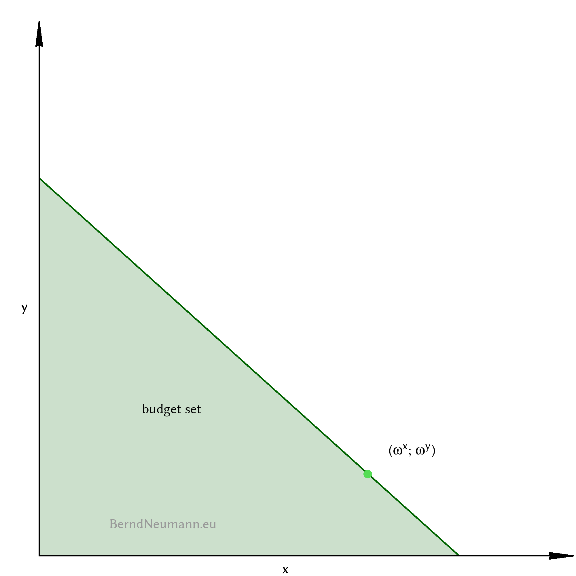
The upper limit of the budget set is the budget line, which is also called the price line in an exchange economy. One obtains its equation by replacing the lower equals sign with an equals sign. It has the slope \(-\frac{p_x}{p_y}\). It intersects with the \(y\)-axis at the position \(\frac{p_x\,\omega^x \;+\; p_y\,\omega^y}{p_y}\), and with the \(x\)-axis at the position \(\frac{p_x\,\omega^x \;+\; p_y\,\omega^y}{p_x}\); i.e. the case where the individual spends his entire income on only one good.

The individual can afford all bundles of goods of the budget set. Of interest are only the bundles on the budget line, because only these bundles can be of maximum utility. Because for every bundle of goods below the budget line there are bundles on the budget line which contain more of all goods and therefore must be better. The individual always spends his entire income on consumption. One must not get the idea that the individual might want to save in order to provide for later consumption. The consumption of goods at different points in time is subject of the theory of intertemporal decision, which is not relevant here nor in the article on exchange economy.

5. The Maximization of Utility

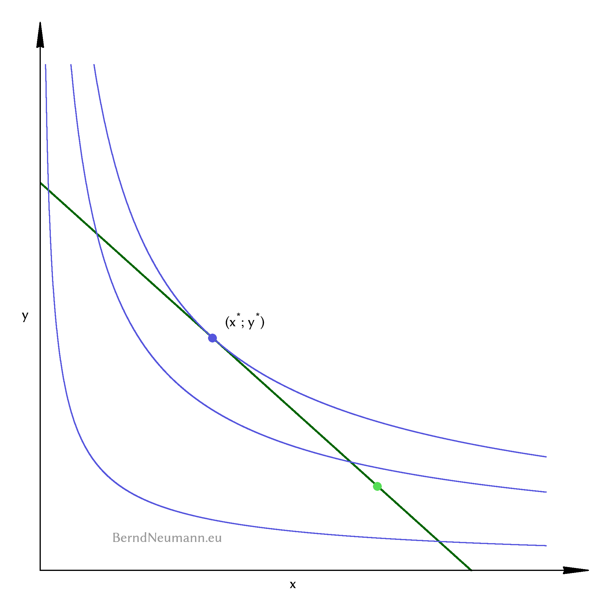
Which bundle of goods will the consumer choose? The answer is first intuitively approached using the diagram in Figure 5. Algebraically, we will solve the maximization of utility in the next section.

Let's choose any bundle of goods within the budget set and draw the corresponding indifference curve. It intersects the budget line at two points, so that the budget set and the better set of this indifference curve form an intersection. The bundles of goods within this intersection are both attainable and better. Therefore we select a bundle of goods from this intersection and draw the corresponding indifference curve again. The picture is similar to the previous one, but our bundle of goods has a higher utility level and the intersection is slightly smaller. We repeat this process until the intersection has disappeared. This is the case if we have selected a bundle of goods right on the budget line whose indifference curve just touches the budget line at the point of this bundle. All other bundles of goods of this indifference curve and all bundles of its better set are outside the budget set. This is the utility maximum bundle of goods that the consumer chooses.

6. The Lagrangian Method

In mathematical terms, the question for the utility maximizing bundle of goods is an optimization problem with a secondary constraint. Fortunately, we do not have to solve this problem ourselves, because Joseph-Louis Lagrange explained a solving method in the middle of the 18th century. It is therefore called Lagrangian method. It is practical that you do not have to understand the mathematics in detail, but only apply the method correctly step by step to solve such an optimization problem.

We first express the optimization problem: We are looking for the maximum value of the utility function \(U(x, y)\), where \(x\) and \(y\) cannot be freely chosen, but must fulfill the budget constraint as a secondary constraint: $$\begin{aligned} &\text{max} \; U(x, y) \; = \; x^{\alpha} \, y^{1-\alpha}\\[1em] &SC: \;\; p_xx \,+\, p_yy \;\leq \; p_x\omega^x \,+\, p_y\omega^y \end{aligned}$$

1. The first step of the Lagrangian method is to set up the Lagrangian function. It consists of the objective function to which the constraint is added, after it has been multiplied with the Lagrange multiplier \(\lambda\) and rearranged to equal zero: $$\begin{aligned} L(x, y, \lambda) \; &= \; x^{\alpha} \, y^{1-\alpha}\\[1em]\;\;\;&+\; \lambda(p_x\,x \,+\, p_y\,y \;-\; p_x\,\omega^x \,-\, p_y\,\omega^y) \end{aligned}$$

2. One forms the partial derivatives of the Lagrange function for all variables and Lagrange multipliers. $$\begin{aligned} \frac{\partial L(x, y, \lambda)}{\partial x} \; &= \; \alpha x^{\alpha-1} \; y^{1-\alpha} \;+\; \lambda\,p_x\\[1em] \frac{\partial L(x, y, \lambda)}{\partial y} \; &= \; x^{\alpha} \; (1-\alpha)\,y^{1-\alpha-1} \;+\; \lambda\,p_y\\[1em] \frac{\partial L(x, y, \lambda)}{\partial \lambda} \; &= \; p_x\;x \;+\; p_y\;y\,-\,p_x\;\omega^x \;-\; p_y\;\omega^y \end{aligned}$$

These derivatives are set to zero, and we write the minus signs in the exponent as fractions: $$\begin{aligned} \frac{\alpha\,x^{\alpha}\,y}{x y^{\alpha}} \;+\; \lambda\,p_x\; &= \; 0\\[1em] \frac{(1-\alpha)\,x^{\alpha}}{y^{\alpha}} \;+\; \lambda\,p_y \; &= \; 0\\[1em] p_x\;x \;+\; p_y\;y\,-\,p_x\;\omega^x \;-\; p_y\;\omega^y \; &= \; 0 \end{aligned}$$

3. One solves the system of equations thus obtained. We eliminate the \(\lambda\) by transforming the first two equations to \((-\lambda)\), equating them and then solving them for \(y\): $$\begin{aligned} \frac{\alpha\,x^{\alpha}\,y}{x y^{\alpha}\,p_x} \; &= \; -\lambda\\[1em] \frac{(1-\alpha)\,x^{\alpha}}{y^{\alpha}\,p_y} \; &= \; -\lambda\\[1em] \frac{\alpha\,x^{\alpha}\,y}{x y^{\alpha}\,p_x} \; &= \; \frac{(1-\alpha)\,x^{\alpha}}{y^{\alpha}\,p_y}\\[1em] y \; &= \; \frac{(1-\alpha)\,x\,p_x}{\alpha\,p_y} \end{aligned}$$

We put this into the third equation (from \(\frac{\partial L}{\partial \lambda}\)) and solve for \(x\): $$\begin{aligned} p_x\;x \;+\; p_y\;\left(\frac{(1-\alpha)\,x\,p_x}{\alpha\,p_y}\right) \; &= \; p_x\;\omega^x \;+\; p_y\;\omega^y\\[1em] p_x\;x \;+\; \frac{(1-\alpha)\,x\,p_x}{\alpha} \; &= \; p_x\;\omega^x \;+\; p_y\;\omega^y\\[1em] x \;+\; \frac{(1-\alpha)\,x}{\alpha} \; &= \; \frac{p_x\;\omega^x \;+\; p_y\;\omega^y}{p_x}\\[1em] \left(\frac{\alpha}{\alpha}+\frac{(1-\alpha)}{\alpha}\right)\,x \; &= \; \frac{p_x\;\omega^x \;+\; p_y\;\omega^y}{p_x}\\[1em] x \; &= \; \frac{\alpha\;(p_x\;\omega^x \;+\; p_y\;\omega^y)}{p_x} \end{aligned}$$

This equation is the solution of the Lagrangian method for the variable \(x\). It tells us, which quantity of good \(X\) the consumer with the initial endowment \((\omega^x; \omega^y)\) chooses to buy at the prices \(p_x\) and \(p_y\) for his maximum utility. – Of interest for everything that follows is how the chosen quantity of good \(x\) responds to different prices. We therefore write it as a function of the prices. This function is the Marshallian demand function. In order to indicate that the quantity of goods is a quantity for maximum utility, we add an asterisk to it. The Marshallian demand function for good \(Y\) is obtained analogously from the equation system of the Lagrangian method: $$\begin{aligned} x^*(p_x, p_y) \; &= \; \frac{\alpha\;(p_x\;\omega^x \;+\; p_y\;\omega^y)}{p_x}\\[1em] y^*(p_x, p_y) \; &= \; \frac{(1-\alpha)\;(p_x\;\omega^x \;+\; p_y\;\omega^y)}{p_y} \end{aligned}$$

The individual thus consumes the bundle of goods \((x^*; y^*)\) and thus maximizes its utility. It is irrelevant how high this utility value is, because it is only relevant that this bundle of goods is the one with the highest utility value within the budget set. This bundle is described by the Marshallian demand functions, and with them everything essential about the decision of a single individual is said.

So far, the analysis only covered the decision of a single individual. One speaks of partial equilibrium analysis. In the article on exchange economy, the aim is to examine the simultaneous actions of several individuals. One speaks then of general equilibrium analysis. Its central concept is presented in the following and last section.

7. The Edgeworth Box

In order to represent the interaction between individuals, a second individual and its diagram of quantities of goods are needed. The first individual is called \(A\), the second one is called \(B\). The utility functions, bundles of goods and Marshallian demand functions are accordingly indexed with \(a\) and \(b\). The diagram of the quantity of goods of \(B\) is not shown on or next to the diagram of \(A\). Instead, the coordinate system of \(B\) is rotated by 180 degrees and its origin is, viewed from \(A\)'s origin, drawn with an offset to the top right. Thus we obtain an Edgeworth box. It represents an economy in which there are certain quantities of both goods, and each point within the box expresses a certain distribution of goods between the individuals. Such a distribution is called allocation.

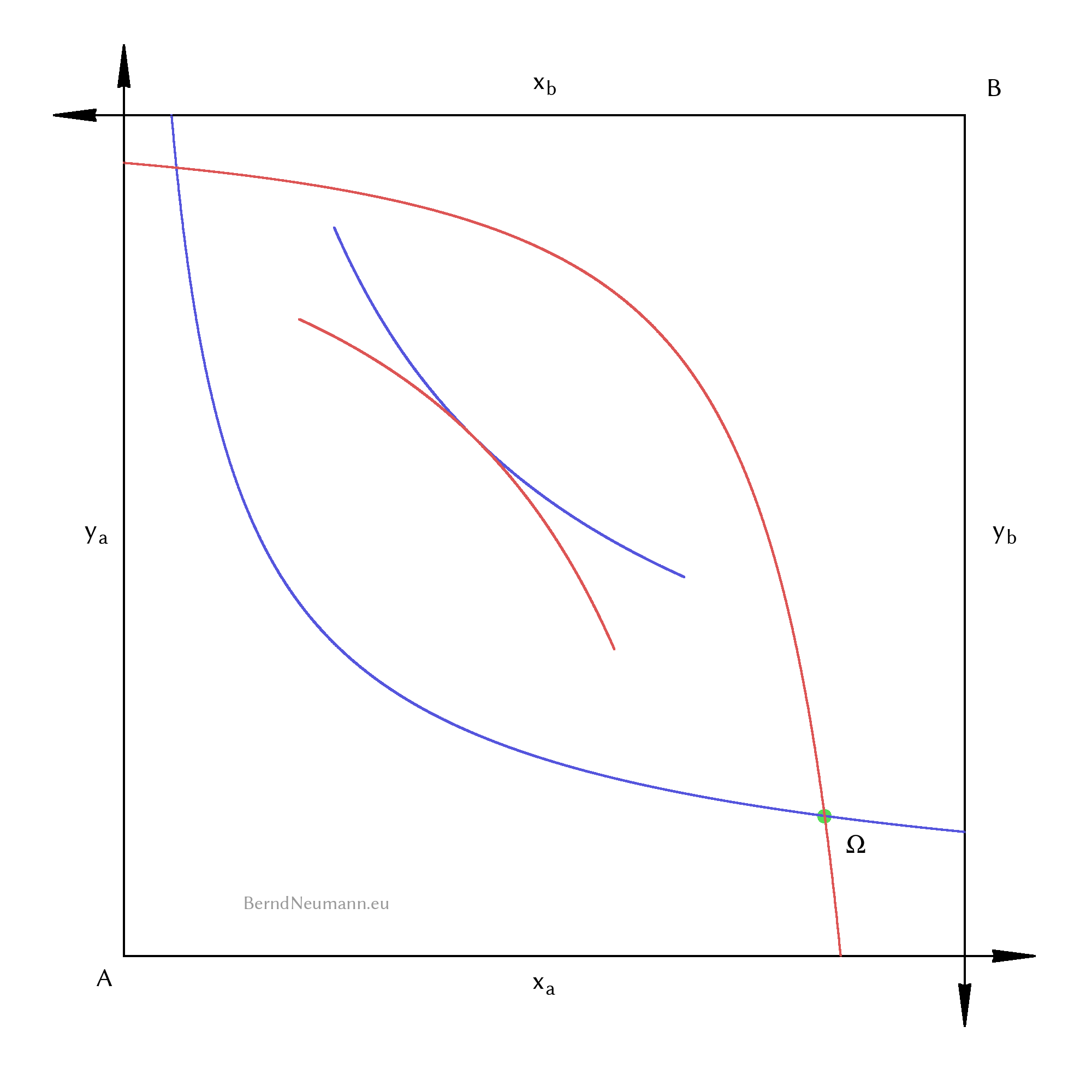
At an allocation further right in the box, individual \(A\) has more of good \(X\); at an allocation further up, more of good \(Y\). Individual \(B\) then has correspondingly less of the respective good. At the point of initial endowment \(\Omega\) individual \(A\) has the bundle \((\omega^x_a; \omega^y_a)\) and individual \(B\) has the bundle \((\omega^x_b; \omega^y_b)\). If one draws the corresponding indifference curves for this allocation, their better sets form a lenticular intersection as common better set. This means that allocations within this intersection are better for both. Thus it is possible to improve the well-being of individuals without having someone lose well-being in return; and it would be inefficient not to do so. In some allocations, there is no such intersection, because there the indifference curves just touch each other. Such an allocation is called a Pareto efficient allocation. There it is no longer possible to make one better off without the other one having to accept a lower utility.

8. Final Remark

In this article 16 terms of microeconomics have been presented. The presentation is not comprehensive, but is intended to serve the propaedeutic purpose of making the article on exchange economy and the First Theorem of Welfare Economics more accessible to the layman. The following list shows the 16 terms:

• Diagram of Quantities of Goods
• Bundle of Goods
• Indifference Curve
• Better Set
• Utility Function
• Cobb-Douglas Utility Function
• Marginal Rate of Substitution
• Budget Set, Budget Constraint
• Budget line, Price line
• Initial Endowment
• Utility Maximization
• Lagrange Method
• Marschallian Demand Function
• Edgeworth Box
• Common Better Set
• Pareto Efficiency

If you have a vivid idea about each of these terms, you know everything necessary to follow the article The exchange economy. At this point it remains to wish you much pleasure.