The three-dimensional Collision of two Spheres

Introduction

What happens when two objects of a given mass, direction and velocity collide? – This is a fundamental question that a physics engine for a physics simulation must answer. However, if one wants to create such an engine and, in view of the fundamental nature of the problem, searches the web in anticipation of good explanations, he will find mainly explanations for certain special and extreme cases, which are of little help in understanding the physics to such an extent that a sufficiently general solution can be implemented with this understanding. Having faced this problem myself, I had some trouble working out the solution. I would like to fill this gap and explain the physics here, derive the necessary equations and offer a possible implementation in C++.

We start with the collision in the one-dimensional space. The goal here is to understand the physics. First, we will get familiar with the elastic and perfectly inelastic collision as limiting cases and derive the equations that describe them. From these limiting cases, we will then determine the general solution of the one-dimensional collision. Then we generalize to the three-dimensional space by formulating the collision in such a way that it can be reduced to the one-dimensional solution (along with a residual part untouched by the collision). This is accomplished through mere vector algebra and adds nothing to the physical understanding. Therefore, it is advantageous to understand the physics in the one-dimensional case. With this knowledge of physics and algebra in three-dimensional space, we will finally write a C++ code that calculates the collision of two spheres. Finally, I will provide a brief insight into the context in which I have engaged with this problem.

This representation is limited in that we will only discuss a central collision, and therefore only talk about spheres. The fact that other objects could get into a rotational motion due to a collision will be negledted in this article. This limitation becomes vivid when considering two elongated objects colliding at their outer ends (and thus not centrally). They will not bounce off each other, but primarily be set into rotational motion. – In presenting the mathematics, I have strived for thoroughness. This may sometimes be tedious for the math expert, but the explicit aim of the presentation is that someone whose knowledge of physics and vector algebra has faded is able to follow the transformations and substitutions without having to fill several sheets of paper.

1. The elastic and the inelastic collision

We are in the one-dimensional space and must first understand two scenarios: Imagine two spheres with equal mass and equal velocity collide head-on. The result of their collision can vary depending on material properties. But all possible outcomes lie between two limiting cases: The first is called an elastic collision. In this case, they bounce off each other and fly away from each other with the same velocity with which they were approaching each other before the collision. In all other cases, they fly away from each other slower than they were approaching each other. This is referred to as an inelastic collision. The second limiting case is that they both come to a stop at the moment of their collision. Then, it is called a completely inelastic collision.

The two limiting cases can be visualized as follows: Consider two perfect rubber balls colliding elastically. If the balls have different masses, you can imagine their elastic collision with a spring between them that stores and then releases their kinetic energy completely during the collision. In contrast, a completely inelastic collision occurs between two sandbags. During their collision, their kinetic energy dissipates into friction (heat) among the sand grains inside the bags. In the one-dimensional case, when the spheres have no motion, unaffected by the collision, this leads to the phenomenon that the objects stick together after the collision. So, they either come to a stop, or they move (sticking together) with the same velocity in the same direction.

Distinguishing between the two limiting cases is pedagogically useful, but it can lead to confusion about the terminology. Therefore, a preemptive remark: We have the completely inelastic collision on one side and the elastic collision on the other. Why isn't the latter limiting case called completely elastic collision? The answer is that the elastic collision is an idealization where no kinetic energy is lost. Physics and mathematics are simpler in this case. Therefore, we will examine this limiting case first. Thereafter we will consider losses of kinetic energy in inelastic collisions. Thus in physics, we don't deal with two ideal types and various mixtures thereof. Instead, it's about simplification (elastic collision) and subsequent generalization, which recognizes the completely inelastic collision as one limiting case and the simplification as the other.

2. The math of the elastic collision

We have two spheres \(A\) and \(B\). They have masses \(m_a\) and \(m_b\) and velocities \(u_a\) and \(u_b\) before the collision. We want to calculate the velocities after the collision \(v_a\) and \(v_b\). For this, we need two physical laws. Firstly, in an elastic collision, we know that the kinetic energy before and after the collision is the same. So, we have: $$\begin{aligned} \frac{1}{2}u_a^2m_a~+~\frac{1}{2}u_b^2m_b ~~&=~~ \frac{1}{2}v_a^2m_a~+~\frac{1}{2}v_b^2m_b \end{aligned}$$

The second law is that of conservation of momentum. It applies to both elastic and every inelastic collision and states that the total momentum (\(mv\)) of the system remains constant. It's important to note that momentum has a direction, so \(v\) and \(u\) are vectors. However, they are easy to handle in the one-dimensional case because the direction of the vector is expressed by the sign. If the spheres are flying towards each other at the same speed, \(u_a\) and \(u_b\) have the same magnitude but different signs. The law of conservation of momentum states: $$\begin{aligned} u_a m_a ~+~ u_b m_b ~~&= ~~ v_a m_a ~+~ v_b m_b \end{aligned}$$

Since the masses and velocities before the collision are given, we have two equations with the two unknowns \(v_a\) and \(v_b\). However, the equation for energy conservation is quadratic, which complicates the solution. Serway and Jewett offer a simple solution where they first eliminate this inconvenience (Serway/Jewett 2008: 257f.). I will follow this solution here with some minor modifications. We simplify the equation for energy conservation by factoring out a term, rearrange it slightly, and apply the third binomial formula: $$\begin{aligned} u_a^2m_a~+~u_b^2m_b ~~&=~~ v_a^2m_a~+~v_b^2m_b\\[1em] m_a~(u_a^2-v_a^2) ~~&=~~ m_b~(v_b^2-u_b^2)\\[1em] m_a~(u_a+v_a)~(u_a-v_a) ~~&=~~ m_b~(v_b+u_b)~(v_b-u_b) \end{aligned}$$

Similarly, we rewrite the equation for conservation of momentum: $$\begin{aligned} m_a~(u_a-v_a) ~~&=~~ m_b~(v_b-u_b) \end{aligned}$$

We divide these two equations and obtain a new equation. Together with the equation for conservation of momentum, we now have a system of equations that is no longer quadratic and much easier to solve: $$\begin{aligned} u_a+v_a ~~&=~~ v_b+u_b\\[1em] v_a m_a ~+~ v_b m_b ~~&= ~~ u_a m_a ~+~ u_b m_b \end{aligned}$$

Rearranging for \(v_a\) and \(v_b\) and substitution yields: $$\begin{aligned} v_a ~~&=~~ \frac{m_a-m_b}{m_a+m_b}~u_a+\frac{2m_b}{m_a+m_b}~u_b\\[1em] v_b ~~&=~~ \frac{2m_a}{m_a+m_b}~u_a+\frac{m_b-m_a}{m_a+m_b}~u_b \end{aligned}$$

Thus, we have calculated the speed and direction, indicated by the sign of \(v_a\) and \(v_b\), of the spheres after the collision, bringing us a little closer to the desired simulation with this first limiting case. Furthermore, we see that the result of a collision is determined by two physical laws: Firstly, the conservation of total momentum, which holds in every case. The second law is the conservation of kinetic energy. It holds completely in this limiting case, and now we turn to cases where the conservation of kinetic energy is only partially fulfilled.

3. The math of the inelastic collision

We know that after a completely inelastic collision, the spheres stick together, meaning they move with the same velocity (and direction). Therefore, we first calculate the completely inelastic collision and then formulate the elastic collision as a mixture of elastic and completely inelastic collisions. For the latter, only the equation for conservation of momentum applies, and the final velocities are equal: $$\begin{aligned} u_a~m_a ~+~ u_b~m_b ~~&=~~ v_a~m_a ~+~ v_b~m_b\\[1em] v_a ~~&=~~ v_b \end{aligned}$$

This we can easily solve: $$\begin{aligned} v_a, v_b ~~&=~~ \frac{u_a~m_a ~+~ u_b~m_b}{m_a~+~m_b} \end{aligned}$$

Thereby, we have determined both limiting cases. Now, we combine these two limiting cases by introducing the parameter \(e\). It determines to what extent the collision is elastic or completely inelastic. We define that \(e=1\) describes an elastic collision while \(e=0\) describes a completely inelastic collision: $$\begin{aligned} v_a ~~&=~~ (1-e)~\frac{u_a~m_a ~+~ u_b~m_b}{m_a~+~m_b}~~+~~e~\left(\frac{m_a-m_b}{m_a+m_b}~u_a+\frac{2m_b}{m_a+m_b}~u_b\right)\\[1em] v_b ~~&=~~ (1-e)~\frac{u_a~m_a ~+~ u_b~m_b}{m_a~+~m_b}~~+~~e~\left(\frac{2m_a}{m_a+m_b}~u_a+\frac{m_b-m_a}{m_a+m_b}~u_b\right) \end{aligned}$$

The common demoninator of the therms is \(m_a+m_b\) and we can simplify to: $$\begin{aligned} v_a ~~&=~~ \frac{u_a m_a + u_b m_b + (u_b -u_a )~m_b~e}{m_a~+~m_b}\\[1em] v_b ~~&=~~ \frac{u_a m_a + u_b m_b + (u_a - u_b)~m_a~e}{m_a ~+~ m_b} \end{aligned}$$

This is the general solution of the inelastic collision along with the limiting cases (elastic and completely inelastic collision). These equations will later appear in the code, determining the length of a component of the motion vector after the collision. However, before we begin with vector algebra for the decomposition of components, we will further complement our understanding of the physics.

4. The coefficient of restitution

We have just introduced \(e\) as a mixing parameter. This corresponds well to the intuition that in inelastic collisions, we deal with mixtures of two extremes. However, \(e\) is not an arbitrary number in \([0;1]\), but has a physical significance. In one-dimensional collisions, it describes the ratio of relative velocities before and after the collision, and it was defined by Isaac Newton in the Philosophiae Naturalis Principia Mathematica, first published in 1687, and is called the coefficient of restitution: $$\begin{aligned} e ~~&=~~ \frac{ v_a - v_b }{ u_b - u_a } \end{aligned}$$

Let me give three additional remarks on this:

i. The general solution for \(v_a\) and \(v_b\) can be derived with the coefficient of restitution and the conservation of momentum. Although this approach is less intuitive than the mixture of the two limiting cases, it is easier to calculate. We solve the definition of the coefficient of restitution for \(v_b\): $$\begin{aligned} v_b ~~&=~~ v_a~-~e~(u_b-u_a) \end{aligned}$$

We substitute this into the equation for the conservation of momentum and solve for \(v_a\): $$\begin{aligned} v_a~m_a ~+~ \left[v_a~-~e~(u_b-u_a)\right]~m_b ~~&=~~ u_a~m_a ~+~ u_b~m_b\\[1em] v_a~m_a ~+~ v_a~m_b~-~e~(u_b-u_a)~m_b ~~&=~~ u_a~m_a ~+~ u_b~m_b\\[1em] v_a ~(m_a~+~m_b) ~~&=~~ u_a~m_a ~+~ u_b~m_b~+~e~(u_b-u_a)~m_b\\[1em] v_a ~~&=~~ \frac{u_a~m_a ~+~ u_b~m_b~+~e~(u_b-u_a)~m_b}{m_a ~+~ m_b} \end{aligned}$$

ii. The coefficient of restitution describes the degree of energy conservation during the collision. This can be illustrated by considering the potential and kinetic energy of a ball that, neglecting air resistance, falls from a certain height to the ground, rebounds, and then springs back up to a certain height. Suppose the ball has the velocity \(v_{before}\) just before impact and the velocity \(v_{after}\) just after. In this case, the coefficient of restitution is the ratio of these velocities: $$\begin{aligned} e ~~&=~~ \frac{v_{nach}}{v_{vor}} \end{aligned}$$

According to these velocities, the ball has kinetic energy just before and after the impact: $$\begin{aligned} E^{k}_{vor} ~~&=~~ \frac{1}{2}~v^2_{vor}~m\\[1em] E^{k}_{nach} ~~&=~~ \frac{1}{2}~v^2_{nach}~m \end{aligned}$$

We rearrange these equations for velocity and substitute them into the equation for the coefficient of restitution: $$\begin{aligned} e ~~&=~~ \frac{\sqrt{\frac{2~E^k_{nach}}{m}}}{\sqrt{\frac{2~E^k_{vor}}{m}}}\\[1em] e ~~&=~~ \sqrt{\frac{E^k_{nach}}{E^k_{vor}}} \end{aligned}$$

Furthermore, we know that the kinetic energy just before impact is equal to the potential energy the ball had at the height from which we dropped it. We call this height \(h_{before}\). Similarly, the kinetic energy just after impact is equal to the potential energy the ball has at the height it reaches after the impact. We call this height \(h_{after}\). For these heights the corresponding potential energy is determined by mass and gravitational acceleration \(g\): $$\begin{aligned} E^p_{vor} ~~&=~~ g~m~h_{vor}\\[1em] E^p_{nach} ~~&=~~ g~m~h_{nach} \end{aligned}$$

In the equation for \(e\), we replace the kinetic energy with its corresponding potential energy and obtain: $$\begin{aligned} e ~~&=~~ \sqrt{\frac{h_{nach}}{h_{vor}}} \end{aligned}$$

This equation vividly illustrates the relationship between the coefficient of restitution and the degree of energy conservation (neglecting air resistance): We drop a ball from height \(h_{before}\), it rebounds and reaches height \(h_{after}\). The coefficient of restitution is then the square root of the ratio of these heights and the associated potential and kinetic energies.

iii. The coefficient of restitution is a property of the collision and not of a specific ball or material. If you drop a rubber ball onto a metal surface, it bounces back almost to its original height. However, if you drop it into a sandbox, it stays put. The coefficient of restitution is also not solely determined by the materials involved. It also depends on the velocity at which the collision occurs. When two metal balls collide at 1 m/s, they undergo an almost elastic collision. However, if they collide at 1000 m/s, it's a completely different scenario. Estimating which coefficient of restitution is effective in a specific collision can be done using tables and approximation formulas. In detail, this requires not only mathematics but also the art of engineering.

5. The decomposition of the velocity vector in the three-dimensional space

We have calculated the result of the collision in the one-dimensional space above. We will now expand this to the three-dimensional space by decomposing the three-dimensional motion vector of the spheres into two components. The first component lies along the line connecting the centers of the spheres. Along this component, we will calculate the collision following the one-dimensional model. We will call this the orthogonal component because it is perpendicular to the tangent plane between the spheres. The second component is perpendicular to the orthogonal component and represents the part of the motion vectors unaffected by the collision of the spheres. We call it the parallel component because it is parallel to the tangent plane.

At the moment of collision, the spheres have position vectors \(\vec{p}_a\) and \(\vec{p}_b\), and the masses \(m_a\) and \(m_b\). We denote the motion vectors before the collision as \(\vec{u}_a\) and \(\vec{u}_b\). The motion vectors after the collision we will denote as \(\vec{v}_a\) and \(\vec{v}_b\), following the same convention as above.

We begin with sphere \(A\). We decompose its motion vector into components expressed as unit vectors multiplied by a scalar. We designate the orthogonal component as \(lao~ \vec{u}^e_{ao}\). Its unit vector will later define the one-dimensional coordinate system in which we calculate the collision. We denote the parallel component as \(lap \vec{u}^e_{ap}\). Let's take a look at the decomposition to visualize right from the start what we aim for: $$\begin{aligned} \vec{u}_a ~~&=~~ l_{ao}~\vec{u}^e_{ao} ~+~ l_{ap}~\vec{u}^e_{ap} \end{aligned}$$

First, we determine the unit vectors. The vector of the orthogonal component points from the center of sphere \(A\) to the center of sphere \(B\). We obtain it by subtracting \(\vec{p}_a\) from \(\vec{p}_b\). To get the unit vector, we need to divide this vector by its length. The length of the vector is the square root of the dot product of this vector with itself. $$\begin{aligned} \vec{u}^e_{ao} ~~&=~~ \frac{\vec{p}_b ~-~ \vec{p}_a}{|~(\vec{p}_b -\vec{p}_a)~|} \end{aligned}$$

Now we need the direction of the parallel component of the motion vector \(\vec{u}_a\) as a unit vector \(\vec{u}^e_{ap}\). For this, we need a helper vector that is perpendicular to the plane defined by \(\vec{u}_a\) and \(\vec{u}^e_{ao}\). We obtain it by taking the cross product of these two vectors. Then, we can take the cross product of this helper vector with \(\vec{u}^e_{ao}\) to obtain the direction of the parallel component.

When dividing by the length of the vector, we must be careful because \(\vec{u}_a\times\vec{u}^e_{ao}=\vec{0}\) may hold, causing the entire numerator to be the zero vector and resulting in division by zero. Geometrically, this occurs, for example, when the spheres collide head-on, or when the motion vector of \(A\) lies precisely on the line connecting the centers of the spheres. Physically, this means that the parallel component is the zero vector. Thus mathematically we must define for this limiting case that \(\vec{u}^e_{ap}=0\): $$\begin{aligned} \vec{u}^e_{ap} ~~&=~~ \frac{(\vec{u}_a~\times~\vec{u}^e_{ao})~\times~\vec{u}^e_{ao}}{|~(\vec{u}_a~\times~\vec{u}^e_{ao})~\times~\vec{u}^e_{ao}~|}~~~~~&\forall~~\vec{u}_a~\times~\vec{u}^e_{ao}~\neq~\vec{0}\\[1em] \vec{u}^e_{ap} ~~&=~~ \vec{0}~~~~~&\forall~~\vec{u}_a~\times~\vec{u}^e_{ao}~=~\vec{0} \end{aligned}$$

We have the directions of the orthogonal and parallel components of the motion vector of \(A\) as unit vectors. Now we need to determine the lengths of these components. We first calculate the length of the orthogonal component. The unit vector of the orthogonal component \(\vec{u}^e_{ao}\) and the motion vector \(\vec{u}_a\) have an inner angle \(\theta\) and an outer angle \(\acute{\theta}\). In the formula handbook we find that we can calculate \(\theta\): $$\begin{aligned} \theta ~~&=~~ \text{cos}^{-1} \left( \frac{\vec{u}^e_{ao} \cdot \vec{u}_a}{|\vec{u}^e_{ao}|~|\vec{u}_a|} \right) \end{aligned}$$

Conveniently, the length of a unit vector always equals to 1, simplifying the formula to: $$\begin{aligned} \theta ~~&=~~ \text{cos}^{-1} \left( \frac{\vec{u}^e_{ao} \cdot \vec{u}_a}{|\vec{u}_a|} \right) \end{aligned}$$

In the argument of the inverse cosine function, we only have vectors known to us, so we could calculate \(\theta\). However, we also know that we can get the length of the orthogonal component \(l_{ao}\) using \(\text{cos}(\theta)\) and the length of the motion vector: $$\begin{aligned} l_{ao} ~~&=~~ \text{cos}(\theta)~| \vec{u}_{a} | \end{aligned}$$

Let us clearify this with a sketch:

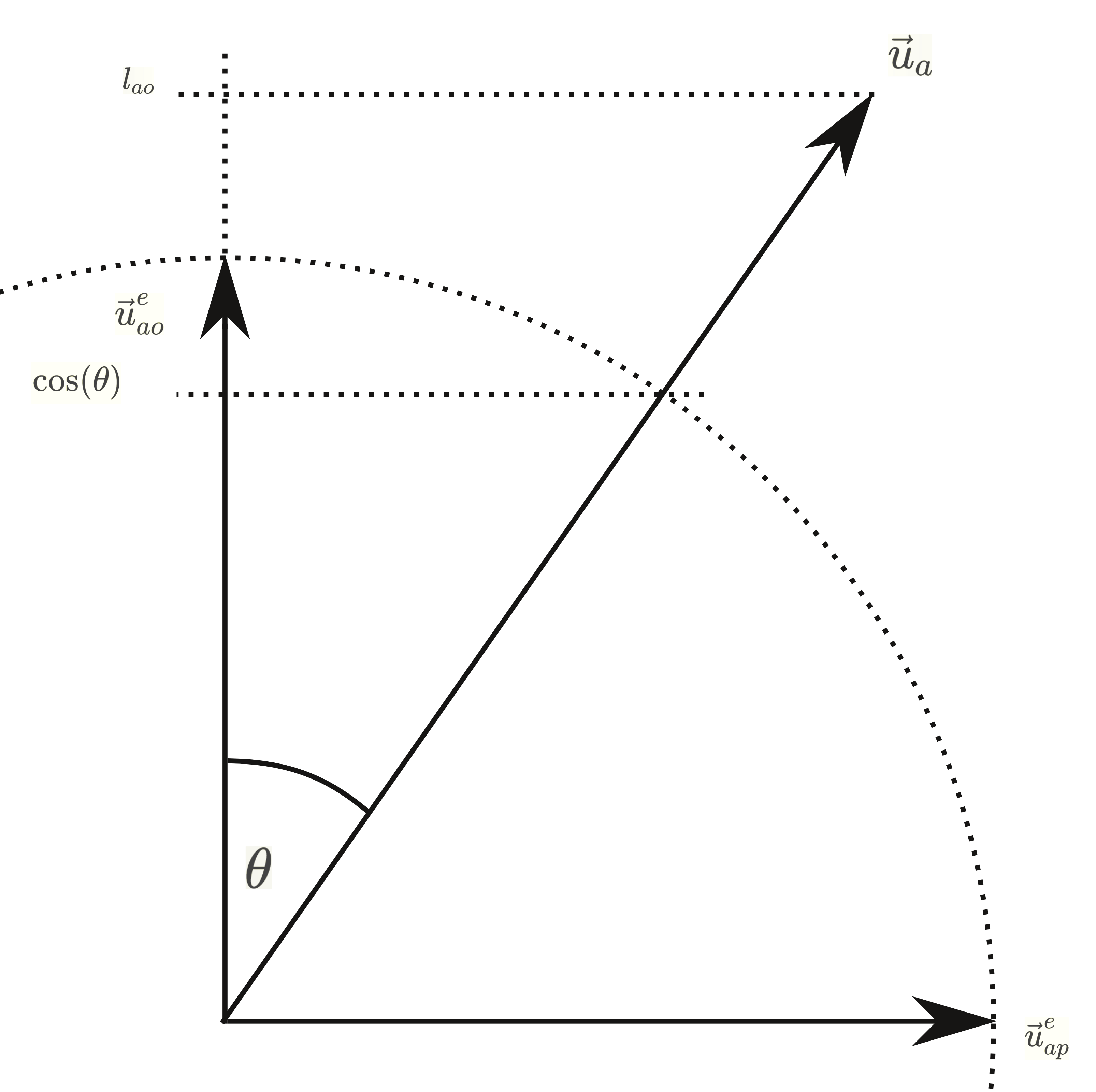
Now we just need to substitute and simplify. We find that the length of the orthogonal component is the dot product of the unit vector and the motion vector: $$\begin{aligned} l_{ao} ~~&=~~ \text{cos}(\theta)~|\vec{u}_{a}|\\[1em] l_{ao} ~~&=~~ \text{cos}\left[\text{cos}^{-1} \left( \frac{\vec{u}^e_{ao} \cdot \vec{u}_a}{|\vec{u}_a|}\right) \right]~|\vec{u}_{a}|\\[1em] l_{ao} ~~&=~~ \vec{u}^e_{ao} \cdot \vec{u}_a \end{aligned}$$

In the same way we get the length of the parallel component as: $$\begin{aligned} l_{ap} ~~&=~~ \vec{u}^e_{ap} \cdot \vec{u}_a \end{aligned}$$

Thus, we have calculated the components of sphere \(A\). Note that the scalar \(l_{ao}\) can also be negative: Suppose a sphere is pushed from behind by a faster sphere. Then, \(\vec{u}^e_{ao}\) points backwards to the center of the pushing sphere, we have \(\theta>90°\), and \(l_{ao}\) becomes negative. This is important because we want to consider the scalars of the orthogonal components (\(l_{ao}\) and \(l_{bo}\)) for the collision as one-dimensional vectors, whose signs must accurately reflect the relative direction of the sphere’s movement.

Hence we should calculate the component decomposition of sphere \(B\) in a way that the scalar \(l_{bo}\) has the correct sign. Therefore, we take the orthogonal unit vector of sphere \(A\) to have both orthogonal components in the same coordinate system (given by \(\vec{u}^e_{ao}\)); instead of calculating an orthogonal unit vector for sphere \(B\) just to obtain a scalar \(l_{bo}\) with a wrong sign that we need to reverse for the collision. Thus, as the component decomposition for sphere \(B\), we are looking for: $$\begin{aligned} \vec{u}_b ~~&=~~ l_{bo}~\vec{u}^e_{ao} ~+~ l_{bp}~\vec{u}^e_{bp} \end{aligned}$$

We take the orthogonal component for sphere \(B\) from sphere \(A\), and thus only need to determine the parallel unit vector for sphere \(B\). Here as well we must take care, because the othogonal component should be the null vector, if the helper vector \((\vec{u}_b~\times~\vec{u}^e_{ao})\) is a null vector: $$\begin{aligned} \vec{u}^e_{bp} ~~&=~~ \frac{(\vec{u}_b~\times~\vec{u}^e_{ao})~\times~\vec{u}^e_{ao}}{|~(\vec{u}_b~\times~\vec{u}^e_{ao})~\times~\vec{u}^e_{ao}~|}~~~~~&\forall~~\vec{u}_b~\times~\vec{u}^e_{ao}~\neq~\vec{0}\\[1em] \vec{u}^e_{bp} ~~&=~~ \vec{0}~~~~~&\forall~~\vec{u}_b~\times~\vec{u}^e_{ao}~=~\vec{0} \end{aligned}$$

A note for deeper understanding: Regarding the parallel component, the difference with sphere \(A\) is that \(\vec{u}^e_{ao}\), from the viewpoint of sphere \(B\), points exactly in the opposite direction of the vector we do not compute for sphere \(B\). Accordingly, \(\vec{u}^e_{bp}\) also points in the opposite direction of the vector we would otherwise have obtained. However, this also reverses the sign of \(l_{bp}\), so that the entire expression \(l_{bp}~\vec{u}^e_{bp}\) accurately represents the parallel component of \(\vec{u}_b\).

Finally we get the scalars of sphere \(B\) analog to sphere \(A\): $$\begin{aligned} l_{bo} ~~&=~~ \vec{u}^e_{ao} \cdot \vec{u}_b\\[1em] l_{bp} ~~&=~~ \vec{u}^e_{bp} \cdot \vec{u}_b \end{aligned}$$

We have now decomposed the motion vectors \(\vec{u}_a\) and \(\vec{u}_b\) into their orthogonal and parallel components. We just need to combine this with the physics from the previous sections to obtain the motion vectors after the collision \(\vec{v}_a\) and \(\vec{v}_b\).

6. The collision

If you've followed along with the physics and mathematics up to this point, you've tackled the greatest challenges. Let's rewrite the result of the component decomposition once again: $$\begin{aligned} \vec{u}_a ~~&=~~ l_{ao}~\vec{u}^e_{ao} ~+~ l_{ap}~\vec{u}^e_{ap}\\[1em] \vec{u}_b ~~&=~~ l_{bo}~\vec{u}^e_{ao} ~+~ l_{bp}~\vec{u}^e_{bp} \end{aligned}$$

Along the direction of \(\vec{u}^e_{ao}\) the collision occurs, with \(l_{ao}\) and \(l_{ao}\) now regarded as the one-dimensional velocity vectors previously denoted as \(u_a\) and \(u_b\). By substituting into the general formula for the inelastic collision, we obtain the three-dimensional motion vectors after the collision: $$\begin{aligned} \vec{v}_a ~~&=~~ \frac{l_{ao} m_a + l_{bo} m_b + (l_{bo} - l_{ao} )~m_b~e}{m_a~+~m_b}~\vec{u}^e_{ao} ~+~ l_{ap}~\vec{u}^e_{ap}\\[1em] \vec{v}_b ~~&=~~ \frac{l_{ao} m_a + l_{bo} m_b + (l_{ao} - l_{bo} )~m_a~e}{m_a~+~m_b}~\vec{u}^e_{ao} ~+~ l_{bp}~\vec{u}^e_{bp} \end{aligned}$$

7. The code (download)

We want to implement these equations as C++ code now. This should be done in the form of a function, to which two objects of the class Sphere are passed by references and the restitution coefficient is passed by value. It is assumed that the function is called when the spheres collide. Similarly, the restitution coefficient is assumed to be given.

We first need a class Sphere that contains all necessary values: These include the position vector, the motion vector, and the mass of the sphere. They are declared as public members within the class to be accessible directly. I limit variables to the ones required for the collision to keep the code simple, thus the class does not contain information about color or material properties, nor does it include the radius. All member variables are declared as double. This ensures not only a decent precision but also faster calculations because modern 64-bit systems typically handle 64-bit floating-point numbers (double) faster than 32-bit floating-point numbers (float).

The function that calculates the collision is declared in collide.h and implemented in collide.cpp. The operation of the physics and mathematics is extensively explained on this page, and the comments in the code should be understood as references to this explanation.

An important note: Those who use this code for simulation purposes must be aware that it only calculates the motion vectors after a collision. A simulation may contain inaccuracies due to its discrete time steps, or floating-point inaccuracies may arise. Balls may slightly overlap during collision, depending on the precision of the simulation. Especially in elastic collisions, it must be ensured that two spheres do not collide and trigger the collide() function again with the new motion vectors. In other words: The spheres must have moved sufficiently apart with their new motion vectors (so they do not intersect anymore) to avoid that collide() is triggered again.

The code is licenced unter the GPLv3 and can be downladed here as a tarball or zip file:

collision.tar.gz
collision.zip

8. Trivia and video examples

Programming is a relaxing pleasure because, especially compared to philosophy, it deals with a clearly defined problem for which one can find a solution that possesses a degree of finality uncommon in philosophy. In this sense, my pursuit of programming does not have a specific application goal; rather, it's simply a way to gain the necessary distance from philosophy at times.

With an object-oriented compiled language like C++, you can relatively quickly develop programs capable of handling complex tasks. As an example, I would like to mention my prime::namespace function templates, which I also offer and document on this website. However, the enjoyment of programming is hindered by the fact that you only get console output and almost have to learn a whole new language to develop a program with graphical output. To shorten this path to graphical output, it seemed obvious to me to program a simulation with C++ that creates scenery files for the ray tracing program povray, which povray then renders into images that can be turned into a movie with ffmpeg. For me, this was the quickest way to go from C++ to moving colorful images that literally visualize the results of my programming efforts. On that account I would like to conclude by showing examples that I created in this way.

Ressourcen

Serway, Raymond A.; Jewett John W. (2008): Physics for Scientists and Engineers with Modern Physics. 9th Edition. Boston 2014. Online bei Archive.org.